Stamm

EXAMPLES OF WORKING WITH DATA
Each of the examples is accompanied by a description and a link to the workbook with the implementation.

Using visual representation of data

Approximation of a complex curve by a polynomial Download

Polynomial dependencies are well suited for approximating complex curves with several inflection points. The Stamm program has a built-in function for finding the coefficients of a polynomial. Below is an example of approximation of an unknown function y=sin(x) by a polynomial. Let's write down 10 pairs of values x and y= sin(x) in columns A and B. Then we insert the function of finding the coefficients of the polynomial in cell D1 (Fig. 9.1).
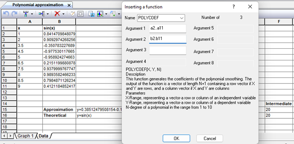
 
Figure 9.1. Inserting the function "POLYCOEFF" to find the coefficients of the polynomial
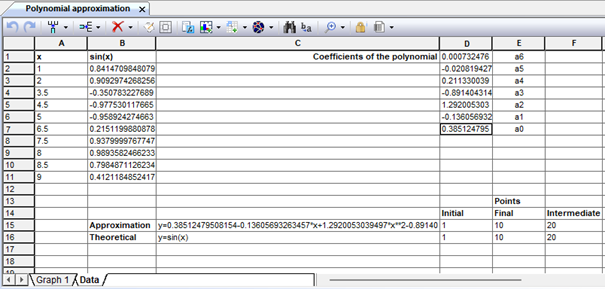
As can be seen from Fig. 9.2, the roots of the polynomial are written in the same way as the approximated data, that is, in a column. It should be noted that the coefficients are written in reverse order, the highest order coefficient is on top, and the free term of the equation is at the bottom. Let's write the resulting polynomial equation in cell C14, and the function y=sin(x) in cell D14.

 
Fig. 9.2. Coefficients and equation of the smoothing curve
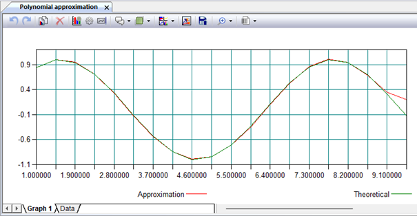
This is necessary to obtain a mapping of both curves on the same graph in order to assess the level of accuracy of the approximation. To the right of the curve equations, we will set the initial and final values of the numerical range X and the number of intermediate points. Having selected a range of equations with parameters in the worksheet, we get a graphical representation of the curves on a separate sheet of the workbook (Fig. 9.3) by selecting the "Graph" button in the "Charts" panel of the "Graphs" tab of the application ribbon. In the resulting graphical representation, the lines and color of the graphs are assigned by default by the system, but if desired, they can be changed using the graph explorer. In the panel of the graphical representation explorer, which is called by double-clicking the left mouse button on the free field of the graph, there are two groups of data, one corresponds to the points of the theoretical curve, and the second corresponds to the points of the approximating dependence. Here, for example, you can create caption legends for graph curves by inserting notes to the corresponding groups, or accentuate the curves themselves by increasing the thickness or color of the lines. How to do this is described in detail in section 5.3.3. It should be noted that after configuring the group styles, it is necessary to set the "All objects in the list" checkbox in the properties panel of the graph component.

 
Figure 9.3. Smoothing the sin(x) function by a 6-order polynomial

As can be seen from Figure 9.3, the curve of the smoothing polynomial dependence has a discrepancy with the theoretical line only at the very end of the range of approximated numerical data.

Analysis of the failure rate of the ignition system Download

For any randomly selected product, it is impossible to determine in advance whether it will be reliable. Failure is an accidental event. Therefore, methods of probability theory and mathematical statistics are used to calculate reliability indicators. One of the conditional concepts used in the calculation of reliability indicators is "operating time". The operating time is the duration or amount of work of the product. For engines, the operating time is usually measured in kilometers of car mileage or in hours (motochas). In the technical and educational literature, you can find such expressions: daily operating time, operating time before the first failure, operating time between failures, etc. Below is an analysis of the failures of the ignition system with a Hall sensor. Experimental data on the operating time of this node are grouped into two blocks: failures in kilometers of the new node and node failures after the first repair, after which numerical data are entered in the workbook data sheet (Fig. 9.4). Moreover, the grouped data does not have to be oriented by rows or columns, so when constructing the frequency distribution, they will automatically be sorted in ascending order.
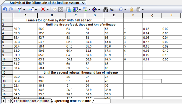
 
Figure 9.4. Data on failures of the ignition system with a Hall sensor in thousand km of mileage
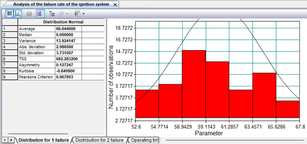
After selecting the desired data block (Fig. 9.4), you can build a histogram of the failure rates of this car node by mileage (Fig. 9.5, 9.6).

 
Figure 9.5. Histogram of failure rates of the new ignition system with Hall sensor (in thousand km of mileage)

 
Figure 9.6. Histogram of failure rates of the ignition system with Hall sensor after the first repair (in thousand km of mileage)

Analysis of histograms allows us to conclude about the maximum probability of failure of this system, which means predicting preventive maintenance of this node.

Predator-prey model Download

This example shows how to solve a differential equation representing a predator-prey model using a tabular model. We use functions for numerical solution of ordinary differential equations using Runge-Kutta integration methods with variable pitch. Consider a pair of first-order ordinary differential equations, known as the Lotka-Volterra equations, or the predator–prey model: dx/dt = x – αxy, dy/dt =−y + βxy. Let's denote x(t) the number of individuals of the prey population, and y(t) — the number of individuals of the predator population at time t. Let also v(t) be the growth rate of the prey population, and w(t) is the growth rate of the predator population. Consider the mathematical model "predator-prey", in which a limited growth model is used for a population of victims. v(t) = (a – bx(t))x(t) – сx(t)y(t); where (a – bx(t))x(t) sets the increase in the number of victims, – cx(t)y(t) – its reduction from being eaten by predators. w(t) = – dy(t) + fx(t)y(t). where – dy(t) sets the reduction in the number of predators due to mortality, fx(t)y(t) – its growth due to feeding by victims. Model parameters: a – coefficient of natural growth of the victim population (a > 0); b – mortality rate of victims from intraspecific competition (b > 0); c – mortality rate of victims from predators (c > 0); d – mortality rate of predators (d > 0); f is the coefficient determining the increase in the number of predators (f > 0). Let's put a blank sheet of a tabular simulation model in the book and create the appropriate cells to simulate population changes.
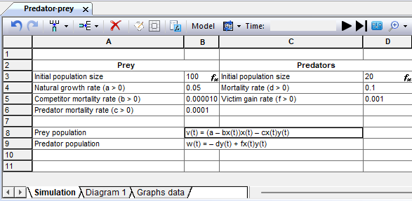
 
Figure 9.7. Sheet for imitation of the Predator-prey model
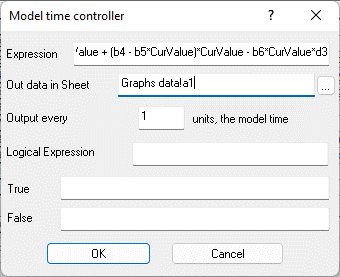
To implement the calculation according to the equations presented above, we will create special cells-controllers B3 and D3 Fig. 9.8 and Fig. 9.9

 
Figure 9.8. Properties of the controller cell to simulate a population of B3 prey
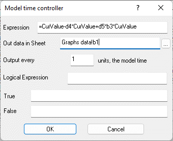
 
Figure 9.9. Properties of a controller cell to simulate a predator population D3
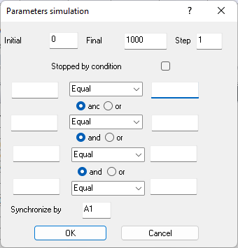
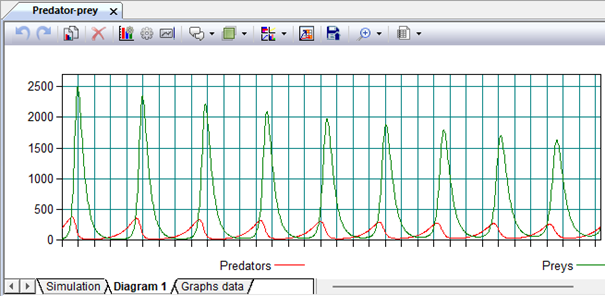
Let's set the initial time to 0 and the time limit in the model parameters panel (Fig. 9.10). After running the model, all intermediate data will be recorded in the "Graph" sheet. To visually display the changes in these data, we will place a special sheet in the book-the diagram "Graph 1" (Fig. 9.11).

 
Figure 9.10. Model Parameters

 
Figure 9.11. Graphical interpretation of the results

Statistical analysis

Forecasting of transportation from the warehouse of an industrial enterprise Download

For the period from 2017 to 2021, the volume of transportation of finished products from the warehouse of an industrial enterprise is known (Table 9.1). It is necessary to make a forecast of the volume of traffic in 2022. Table 9.1 Traffic volumes by year Period (year) 2017 2018 2019 2020 2021 Sales volume (thousand tons) 320 470 540 710 1025 Let's create a sheet with initial data in the workbook (Fig. 9.7).
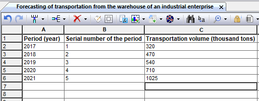
 
Fig. 1. A sheet with initial data on traffic volumes

Let's build a graph of changes in traffic volumes by year, for which we will select the "Graph" option - "Simple" from the drop-down menu of the rightmost button of the current sheet (Fig. 9.8) and set the plot points (Fig. 9.9).

 
Fig. 2. The menu for selecting the type of graph
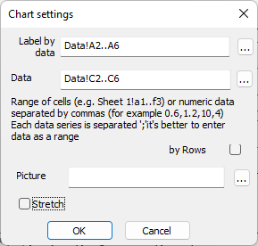
 
Fig. 3. Chart data range
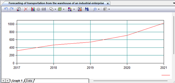
 
Fig. 4. Sketch schedule of traffic volume changes
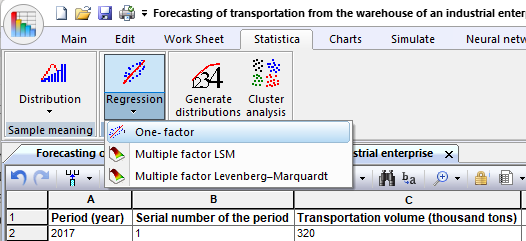
The demand curve shows that a linear model can be used to determine the function of the dependence of the volume of traffic by calendar years. Let's try to find a linear regression model describing the trend of traffic volume changes over the years, of the form y=a+b·(x). To do this, use the drop-down menu in the "Statistics" section of the application feed in which we select the "Simple regression" option (Fig. 9.11).

 
Fig. 5. Menu of the "Statistics" panel of the application feed

Or by selecting the appropriate option "Statistics" - "Regression" - "Simple" from the drop-down menu, the rightmost toolbar button of the current sheet (Fig. 6).

 
Fig. 6. Menu of the dashboard of the worksheet
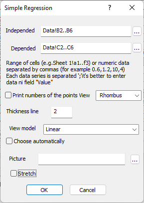
Let's set the ranges of experimental points and the type of regression dependence (Fig. 7).

 
Fig. 7. Regression dependence settings panel
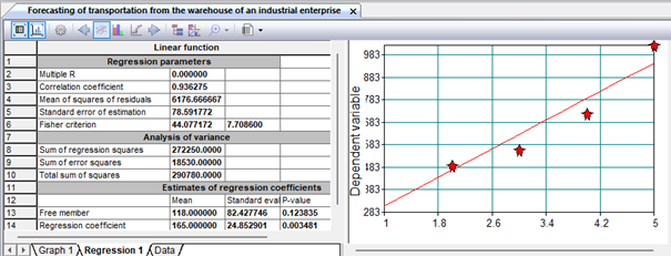
 
Fig. 8. Regression dependence parameters
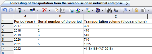
Let's enter the regression equation in the cell opposite the planned period and try to get a forecast value of traffic volume for 2022 (Fig. 9).

 
Fig. 9. Calculation of the regression dependence in the cell
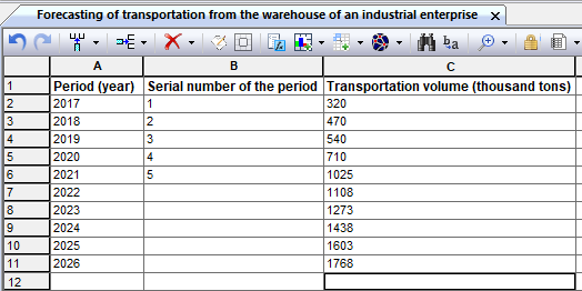
After that, we copy the formula into the corresponding cells below the last reporting year and get similar values for five prospective years (Fig. 10).

 
Fig. 10. Calculation of the traffic forecast for the prospective period

Obtaining parameters of multivariate regression dependence of the annual turnover of small enterprises on their characteristics by regions of Russia Download

The Internet provides statistical data on the indicators of small enterprises in the regions of Russia. Let's assume a linear view of the dependence of the turnover of small enterprises on their number in the region and the average number of employees. Let's perform a multivariate regression analysis using a linear mathematical model on the main effects in the Stamm system. Let's transfer the data to the Stamm worksheet (Fig. 9.100).
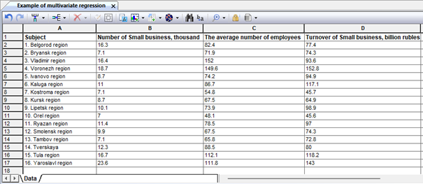
 
Figure 1. Initial experimental data
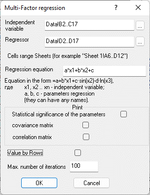
On the "Statistics" tab of the application ribbon, select the button with the "Regression" drop-down menu, and from the drop-down menu list, select the "Levenberg-Marquadt Multivariate" option. Or open the menu of the leftmost toolbar button of the current sheet in accordance with the nesting shown in Fig. 9.97a. Let's adjust the regression parameters as indicated in the previous example, but taking into account the selected linear dependence (Fig. 2). The results of approximation by the given formula are shown in Fig. 3 - 8. They show that parameter estimates for independent variables have almost the same elasticity coefficients, which indicates an approximately equal influence of factors on the response function. The coefficients of multiple correlation and determination are quite high, that is, the regression with the obtained parameters satisfactorily approximates the studied dependence. At the same time, the standard error is very high, which is due, on the one hand, to insufficient sample size, and possibly an incorrect choice of theoretical dependence.

 
Figure 2. Regression analysis parameters panel
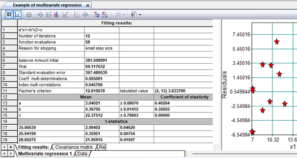
 
Figure 3. Approximation results
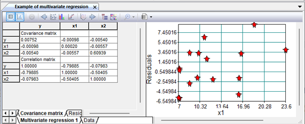
 
Figure 4. Approximation results
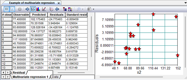
 
Figure 5. Covariance and correlation matrices
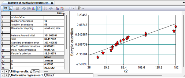
 
Figure 6. Residuals of the model
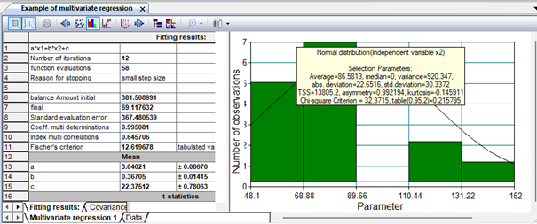
 
Figure 7. Estimation of the normality of the distribution using probability paper

 
Figure 8. Estimation of the normality of the distribution using the distribution function

The results of the analysis of the normality of the distribution of variables show that the coefficient of asymmetry of the distribution is quite high (fig. 8), which may indicate an insufficient sample size.

Using simulation models of tabular type

Modeling of expenses related to car sales in the salon Download

The following example from the practice of a car dealership is posted on the Internet. In the last hundred months, the sales volume at the dealership ranges from 5 to 11 new cars per month. The salon manager orders 25 cars each time and makes a new order when the stock in the store is reduced to 10 cars. A new order can be made only after the previous one has been completed. We will simulate this strategy for 24 months. Let's perform a Monte Carlo simulation by setting car sales for a month by a random number with the given parameters of the distribution law.
We believe that:
a) the initial stock is 30 cars
b) the cost of storing one car is 550,000 rubles per month.
c) one missed sale brings an average loss of 3,330,000 rubles.
d) one order costs 500,000 rubles.
Modeling tasks:
1. How many orders will have to be made in two years?
2. What are the costs associated with this strategy (thousand rubles)?
Let's create a new workbook and insert a simulation sheet there. Let's call it "Imitation of sales". In this sheet, we will create 6 special controller cells necessary for sales modeling (Fig. 9.12).
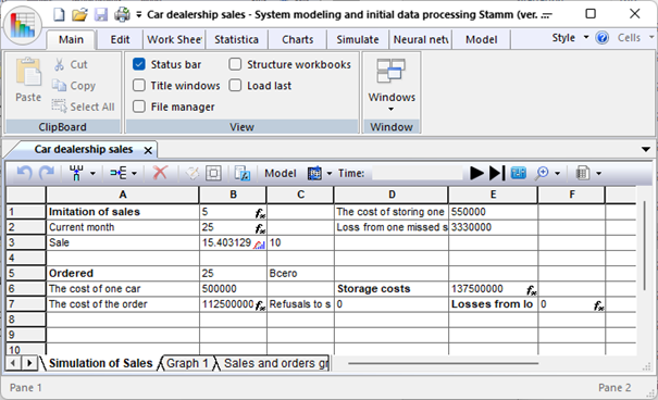
 
Figure 9.12. Simulation sheet for sales modelling
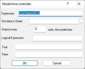
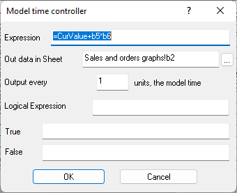
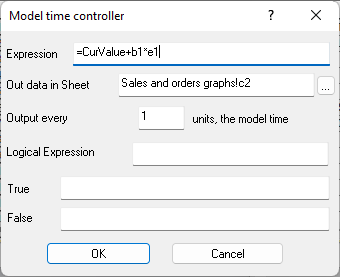
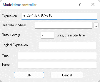
The first cell B1 – controller "Calculated expression" is designed to simulate the number of cars of this brand in the cabin. The properties of the cell are shown in Figure 9.13.

 
Figure 2. Formula in cell B1

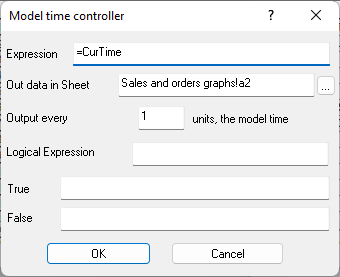
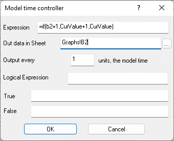
All special cells are recalculated at each iteration, that is, the change of the calendar month. At the same time, the number of ordered cars is added to the current value in cell B1, if there is an order, and the number of cars sold, generated randomly, is subtracted. Cell B2 – controller "Calculated expression" is designed to set the value of the current month. The properties of the cell are shown in Fig. 9.14.

 
Figure 9.14. Formula in cell B2

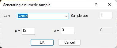
Cell B3 – controller "Random variable Generator" is designed to simulate the sales of the current month. The properties of the cell are shown in Fig. 9.15. The cell will be a generator of a random value of sales in the current month, which is subject to the normal law with the parameters expectation - 12 and variance 3.

 
Figure 9.15. Formula in cell B3

Cell B7 – controller "Calculated expression" is designed to simulate the costs of ordering cars. The properties of the cell are shown in Fig. 9.16.

 
Figure 9.16. Formula in cell B7

Cell E6 is designed to simulate the cost of storing cars in the cabin. The properties of the cell are shown in Fig. 9.17.

 
Figure 9.17. Formula in cell E6

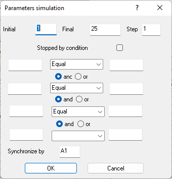
The last special cell F7 is designed to simulate losses from the refusal to sell a car. The properties of the cell are shown in Fig. 9.18. The model parameters are set via the dialog panel (Fig. 9.19). At the same time, the current month is used as a model time variable, respectively, the modeling step is 1. In order to simulate the operation of the salon for two years, the final value is set to 25, when it is reached, the simulation stops.

 
Figure 9.18. Formula in cell F7

 
Figure 9.19. Model Parameters
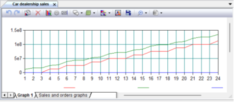
In the properties of the cells that store the values of the current month and accumulated costs, the output of numerical values is set at each step of the modeling in the workbook "Sales and Order Schedules" (Fig. 9.16 – 9.18). Accordingly, after the end of the model, you can select a data block in this sheet to get a graph of cost changes by elements on a separate graphical representation (Fig. 9.20). The operation of the model stops when the specified model period is reached (Fig. 9.21).

 
Figure 9.20. Cost change graphs

 
Figure 9.21. Simulation results

Modeling of repair of mechanisms in the workshop Download

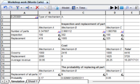
The repair shop performs preventive inspection and repair of some mechanisms. Of all the mechanisms received by the repair service, 30% are mechanisms of type A, 50% – type B, 20% – type C. The mechanism of type A includes 10 parts that require inspection; the mechanism of type B includes six such parts, type C – four parts. The number of parts requiring replacement in each of the mechanisms can be any. For example, in a type A mechanism, the number of parts requiring replacement can range from 0 to 10 (with the same probability). For each replaced part, the customer pays the repair shop 5 den. units. In addition, the customer pays 10 monetary units for the inspection of mechanism A. units, for the inspection of the mechanism B – 8 monetary units, for the inspection of the mechanism C – 14 monetary units. Create an algorithm and a program (based on the Monte Carlo method) to determine the following values: – the probability that all parts will need to be replaced in the mechanism; – the average revenue of the workshop from the inspection and repair of one mechanism. The problem was solved using a macro written in VBA for Excel, implementing the Monte Carlo method. The implementation of this task in the Stamm system is presented below. The simulation sheet of the corresponding workbook contains 4 controller cells, which are random number generators distributed according to a given law, and 9 controller cells "Calculated expression" (Fig. 9.22).
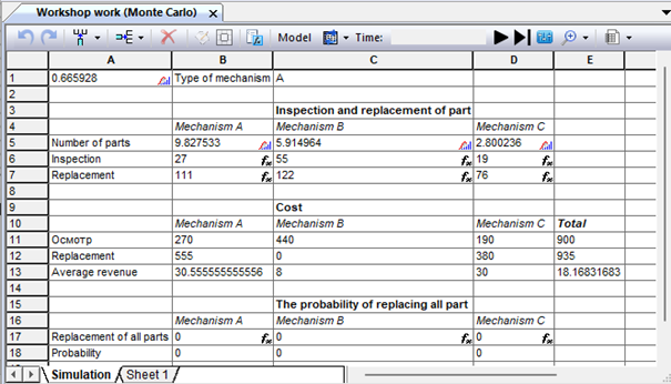
 
Figure 9.22. The sheet of simulation of inspections and replacement of parts
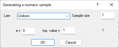
Cell B1 generates a uniformly distributed random variable in the range from 0 to 1.

 
Figure 9.23. Controller cell B1

After that, the formula in cell C1 selects the mechanism code depending on the value of the variable generated in B1 =IF(A1<0.3,"A",IF(A1<0.8,"B","C")) Depending on the code received as a result of the iteration, one of the controller cells increases the counter of the mechanisms received for inspection by one. Figure 9.24 shows cell B6, which is responsible for counting the number of examined type A mechanisms.

 
Figure 9.24. Formula in cell B6

Cells C6 and D6 contain similar formulas and are responsible, respectively, for counting the number of examined mechanisms of type B and C. Replacement of parts for each type of mechanism is imitated by cells B7, C7, D7 using the same type of formulas (Fig. 9.25), increasing the value in the cells for their type. And the number of replaced parts by types of mechanisms is generated in cells B5, C5, D5 according to the same uniform distribution law (see Fig. 9.26).

 
Figure 9.25. Formula expression in cell B7
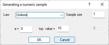
 
Figure 9.26. Generation of a random variable in cell B5
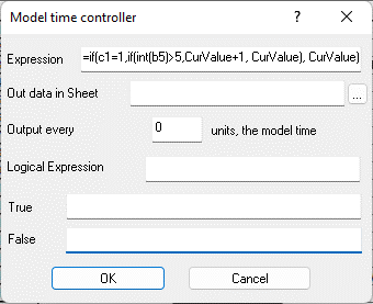
Cells B17, C17 and D17 track the number of replaced parts generated in cells B5, C5, D5, compare it with the maximum number of parts in the mechanism of the corresponding type and increase the counters of complete replacement by types of mechanisms (Fig. 9.27).

 
Figure 9.27. Formula in cell B17

 
Fig. 9.28. Simulation results

Formulas in ordinary cells of the sheet use the values generated during the simulation to calculate the necessary indicators. Calculation of the cost of inspection of mechanisms by types A, B, C is carried out in cells B11, C11 and D11 according to the formulas, respectively: =10 *B6, =8*C6, =10*D6. The cost of replacing parts by types of mechanisms is calculated in cells B12, C12 and D12 according to the formulas: =5*B7, =5*B7, =5*D7. The average revenue from the mechanisms for the simulated period is calculated in cells: =(B11+B12)/B6, =(C11+C12)/C6, =(D11+D12)/D6. And finally, the probability of a complete replacement is calculated based on the number of complete replacements of parts by type of mechanisms and the total number of inspections of mechanisms of each type according to the formulas: =B17/B6, =C17/C6, =D17/D6.

Determination of the optimal fleet of vehicles for the delivery of goods from the wholesale base Download

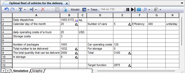
Several variants of such a task are presented on the Internet, in general, its formulation is as follows. From the wholesale base, the products go on retail sale. Consumers are located in the city, where the wholesale base is located. The products received at the wholesale base should be processed and, if possible, delivered to consumers on the same day. If it is not fully exported, it remains at the base, thus creating losses associated with its storage. For simplicity, it is assumed that the auto enterprise and the base work seven days a week. The distance from the wholesale base to consumers is not set, but it is known that each of the machines can take out a given amount of cargo. The flow of products entering the wholesale base obeys the normal law of distribution. It is required to determine the optimal size of the fleet of machines needed to deliver products from the wholesale base to consumers. The criterion of optimality is the minimization of total costs, consisting of the costs of operating vehicles and the costs of cargo storage. The consumer service system is a discrete type system with a jump-like transition from one state to another at any event. For example, by changing the number of cars, you can change the cost of transporting goods, the speed of their delivery. The flow of incoming goods is irregular, therefore, the optimal ratio between cost groups can be established by selecting the law of management of service facilities (machines), and all the necessary values can be found analytically, without experiment. This analysis can be performed using the Monte Carlo method, which is the application of the procedure of "unlimited random sampling" of individual elements on a set in such a way that the probability of sampling each element is the same. The method is a simulation of an experiment to determine the probabilistic properties of a set of events. We will find such an optimal number of machines servicing the base, at which the total costs of transportation and storage will be minimal. The simulation sheet of the corresponding workbook contains one controller cell, which is a generator of random numbers distributed according to a given law, and 6 controller cells "Calculated expression" (Fig. 9.29).
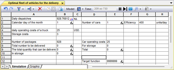
 
Figure 9.29. Modeling sheet of the optimal number of vehicles for the export of products
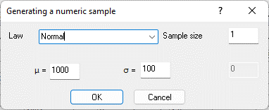
Cell B1 generates the daily amount of cargo receipt to the wholesale base - a random variable distributed according to the normal law with an average value of 1000 and a standard deviation of 100.

 
Figure 9.30. Controller cell B1

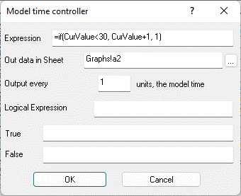
After that, the generated number is rounded in cell B7 using the built-in formula "=INT(B1)" and used in further modeling. The "Calculated Expression" controller cells - B2 and E2 are designed, respectively, to generate the current day of the month and the number of working cars (Fig. 9.31, 9.32). The current day of the month is calculated using a simplified function, since this is not critical for the Monte Carlo method. To analyze the simulation results, the output of numerical data of these cells is provided in columns A and B of the "Graphs" sheet. It should be noted that the fields of these cells with links to output to a given sheet can be used as non-modal (see the description of non-modal windows above).

 
Figure 9.31. Formula in cell B2

 
Figure 9.32. Formula in cell E2
Cells B4 and B5 contain constants corresponding to the cost of operating cars and the costs associated with storage on the basis of a unit of production. Cell G2 stores the average performance of one car as a random value (Fig. 9.33). Based on this value, cell B9 calculates the amount of products that can be delivered from the base to consumers during the working day by all cars according to the equation "=E2*G2". The total number of products to be delivered is modeled in cell B8 (Fig. 9.34), and not exported and left for storage after the work shift - in B10 (Fig. 9.35).

 
Figure 9.33. Formula in cell G2

 
Figure 9.34. Formula in cell B8
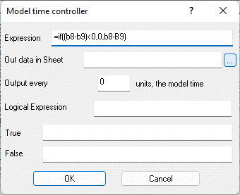
 
Figure 9.35. Formula in cell B10
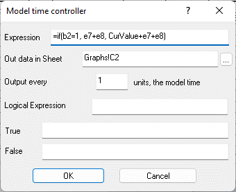
The costs of operating cars and storing products in a warehouse are determined in cells E7 and E8 according to the formulas, respectively, "=B4*E2" and "=B5*B10". The total costs associated with the export of products are reset at the beginning of each month, and then accumulated during the modeling process, the E9 controller cell is responsible for this (see Figure 9.36).

 
Figure 9.36. Formula expression in cell E9
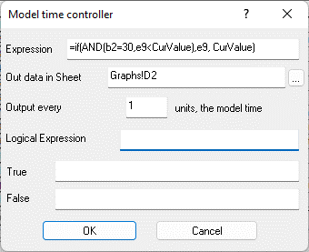
Cell E12 is an objective function, it serves to check optimality after each iteration and contains a logical expression based on the built-in functions of the formula processor (Fig. 9.37). Before starting the simulation, the maximum possible number is entered into it. After modeling a month of operation of a certain number of cars, if the total costs are less than the value of the objective function, then its value is assumed to be equal to these costs.

 
Рис. 9.37. Формула в ячейке E12

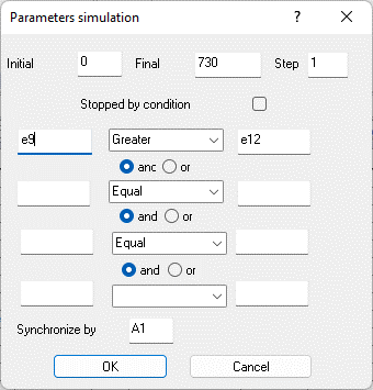
The model parameters are set via the dialog panel (Fig. 9.38). At the same time, the final value is set to a number that allows you to simulate the operation of cars for two years, with a modeling step equal to 1. Unlike the previous examples, the simulation stops if the value of the total costs (cell E9) after the next iteration becomes larger than the target function in cell E12, this is set by the corresponding condition in the dialog panel.

 
Figure 9.38. Model parameters

As a result of running the model with the specified parameters, it turns out that the optimal number of cars for the export of products is 5 (Fig. 9.39).

 
Figure 9.39. Simulation results

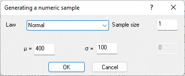
If you set the output of the car per shift not by a constant value, but by a random one, for example, the average 400 and the standard deviation, taking into account the influence of various factors (Fig. 9.40), then the result of modeling with a standard deviation of 100 will already be somewhat different (Fig. 9.41).

 
Fig. 9.40. Generation of a random output value in cell G2
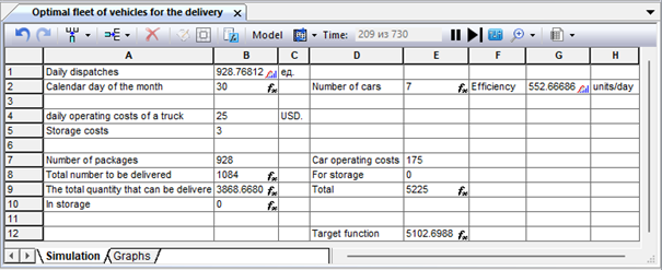
 
Fig. 9.41. The results of the model operation with the random nature of the car production
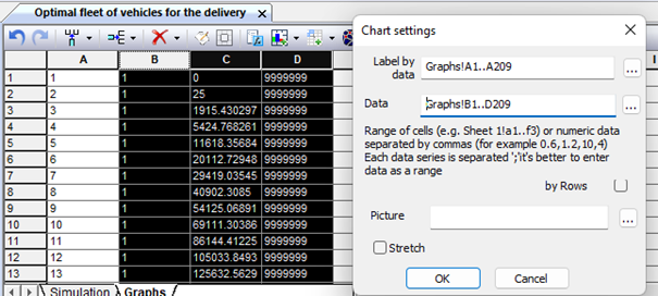
Let's plot the change graphs of the objective function and the total transportation costs, based on the numerical values stored in the modeling process in the "Graphs" sheet (Fig. 9.42).

 
Fig. 9.42. Selecting data for plotting cost changes
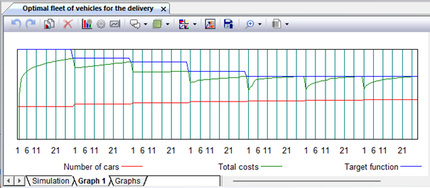
Since the numerical values of the parameters differ significantly during modeling, for example, we set a deliberately large initial value for the objective function, we use a logarithmic scale in the display settings (Fig. 9.43). To display the legend, we will create text annotations for all data series.

 
Fig. 9.43. Schedule of changes in delivery costs

Simulation of fuel consumption using a driving cycle profile Download

For some brands and models of cars, the dependences of the engine fuel efficiency indicators on the crankshaft rotation speed, load and other engine characteristics have been investigated and numerical values of the parameters of these dependences have been experimentally established. These dependencies are written in the language of the formula processor "Stamm", similar to ordinary equations, with the exception of variable references to other cells. When removing the speed and load profile of a typical driving cycle for a given make and model of car, it becomes possible to create models to simulate fuel consumption under the influence of various external conditions, for example, ambient air temperature, duration of stops with the engine running, etc. The speed and load profile of the driving cycles are set in tabular form in the form of a vector of values, the first coordinate of which is the time from the start of the cycle, and the second and subsequent parameters of the car are speed, crankshaft speed, throttle opening degree, etc. The speed profile of the driving cycle is set in a regular workbook sheet (Fig. 9.53).
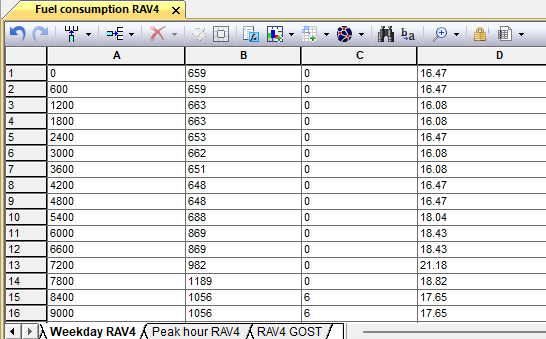
 
Fig. 9.53. Speed profile "Urban driving cycle"
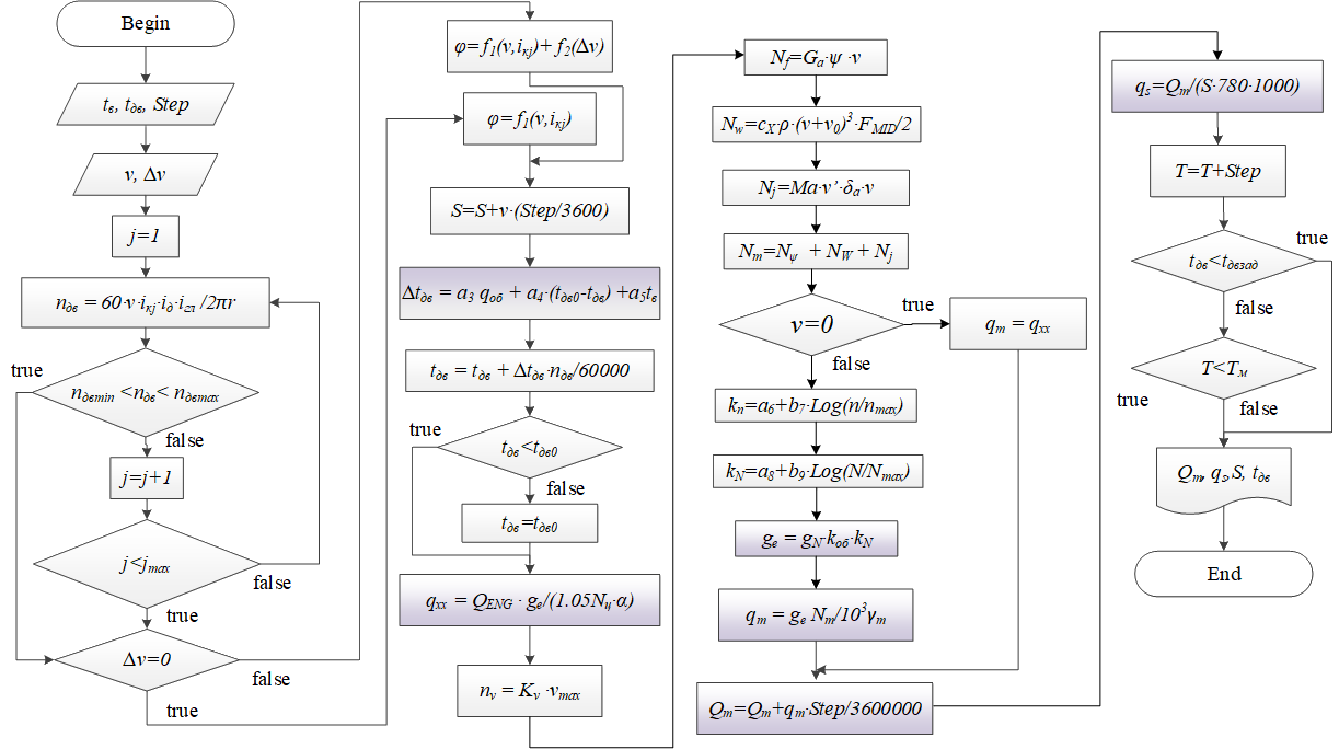
The general algorithm of the simulation model of fuel consumption using the profile of the driving cycle is shown in Fig. 9.54.

 
Fig. 9.54. Algorithm of the simulation model based on the profile of the driving cycle
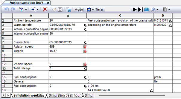
The model of fuel consumption when driving a car on a driving cycle for a Toyota RAV4 with a 2000 cm3 engine and automatic transmission, implemented in the Stamm system, is shown in Fig. 9.55.

 
Fig. 9.55. Workbook "Modeling of fuel consumption"
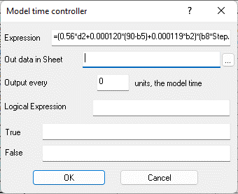
The simulation sheet contains the "Calculated Expression" controller cells for calculating the parameters of the car and engine according to dependencies, the numerical values of which were obtained experimentally (cells B3 and D2, D3). Figure 9.56 shows the properties of the controller cell D2, reproducing the dependence of fuel consumption per revolution of the crankshaft of the internal combustion engine on the load on the engine and the rotational speed of the crankshaft of the engine.

 
Fig. 9.56. Properties of the controller cell "Calculated expression" B3
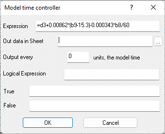
Fig. 9.57 displays the properties of the B2 controller cell, which simulates the dependence of fuel consumption per revolution of the engine crankshaft on the load on the engine and the speed of rotation of its crankshaft.

 
Fig. 9.57. Properties of the controller cell "Calculated expression" D2
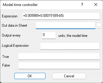
A cell of a similar type D3 simulates the pattern of changes in the fuel consumption per revolution of the engine crankshaft from the coolant temperature (Fig. 9.58).

 
Fig. 9.58. Properties of the controller cell "Calculated expression" D3
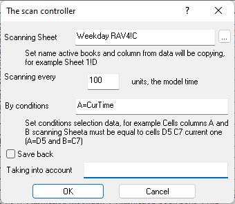
Reproduction of the parameters of the driving cycle in the simulation model corresponding to the model time is carried out by special cells "Scan Controller". In Fig. 9.59 the properties of a cell of this type designed to reproduce the speed of the car corresponding to the current model time are presented.

 
Fig. 9.59. Properties of the "Scan Controller" cell B12
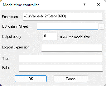
Cell B13 contains a calculated expression that simulates an increase in the mileage of a car, taking into account the speed and step of the simulation (Fig. 9.60).

 
Fig. 9.60. Properties of the controller cell "Calculated expression" B13
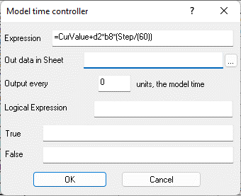
The controller cell B14 is designed to calculate the value of the total fuel consumption during the simulation (Fig. 9.61).

 
Fig. 9.61. Properties of the controller cell "Calculated expression" B14
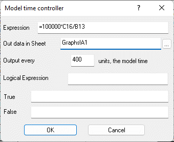
Cells C15 and C16 containing the formulas "=B15/1000" and "=C15/780", respectively, are responsible for converting the obtained flow values into grams and liters. The value of the specific fuel consumption in the model is reproduced by cell C17 (Fig. 9.62). The numerical values obtained during the simulation of the current fuel consumption are displayed in a separate sheet of the workbook "Graphs".

 
Fig. 9.62. Properties of the "Calculated expression" cell C17
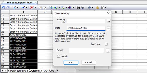
After creating and configuring all the cells of the simulation sheet in accordance with the model algorithm (Fig. 9.54), it is possible to simulate fuel consumption when driving a RAV4 car outside the city, for example, at different ambient temperatures. The data obtained during the simulation can be used to plot changes in the fuel efficiency of the car while driving (Fig. 9. 64), when determining the range of cells for displaying the curve, it must be taken into account that at the beginning of the simulation, fuel consumption can be reset and there will be an indefinite value in cell C17 (Fig. 9.63).

 
Fig. 9.63. Setting the chart parameters. Selecting a data range
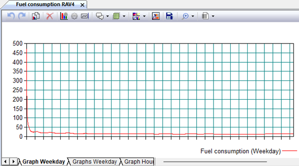
 
Fig. 9.64. Schedule of fuel consumption changes during simulation (Weekdays)
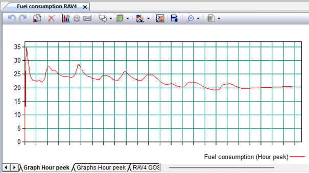
Such high fuel consumption values at the beginning of the experiment are due to the stopping of the car and the lack of mileage when performing a simulation experiment on the speed profile of the driving cycle "Weekdays". If we simulate traffic on the "Rush Hour" profile, where there is no stop at the beginning of the speed profile, we will get a different form of the graph (Fig. 9. 65).

 
Fig. 9.65. Schedule of fuel consumption changes during simulation (Hour peek)

Simulation of the thermal state of the engine when warming up at idle Download

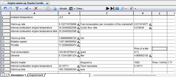
A simulation model of the process of warming up an automobile engine can be useful in determining the duration of warming up to a certain temperature of the coolant at a given ambient temperature and a different initial value. To obtain the amount of fuel consumption consumed for heating at idle under various external conditions. At the same time, the model does not use time profiles, although the value of the model time itself and its increment step are used for numerical integration when calculating the warm-up time, fuel consumption and some engine parameters. The sheet of the simulation model of the internal combustion engine heating is shown in Fig. 9.66. In the process of simulating idling, the engine operation mode is reproduced, set by the injection control controller of a real engine. This is achieved using experimentally obtained regression dependencies: the speed of rotation of the crankshaft and the degree of throttle opening on the temperature of the coolant and the external environment. These dependencies are implemented in cells B8 and B9 (Fig. 9.67, 9.68).
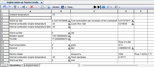
 
Fig. 9.66. Workbook "Warming up the Toyota Corolla internal combustion engine"
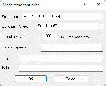
 
Fig. 9.67. Properties of the cell "Calculated expression" B8
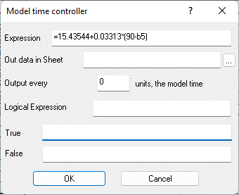
 
Fig. 9.68. Properties of cell B9
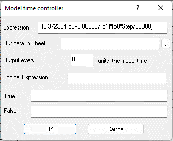
With the help of experimental studies of the operation of the engine of a real car at idle, the form of equations and numerical values of their parameters were also obtained for calculating the rate of heating of the coolant and the specific fuel consumption per revolution of the crankshaft (Fig. 9.69, 9.70).

 
Fig. 9.69. Cell B3 "Calculated expression" - the rate of heating of the internal combustion engine coolant
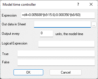
 
Fig. 9.70. Cell D3 "Calculated expression" - fuel consumption per revolution of the engine crankshaft
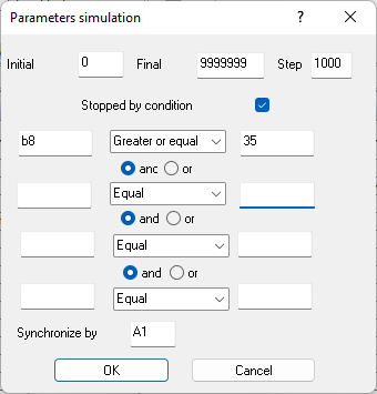
By changing the values in the cells of the simulation sheet, for example, the ambient temperature – B2 and by setting simulation conditions using the model parameters panel (Fig. 9.71), it is possible to simulate warm-up indicators in various conditions. For example, in Fig. 9.71, the limit value of the coolant temperature (35oC) is set, at which the simulation stops. If we first reset the values of the warm-up time and total fuel consumption in cells B7 and B11 and set the value of the external environment in cell B2 of the simulation sheet, then as a result we will get the time needed to warm up to the specified temperature (Fig. 9.72).

 
Fig. 9.71. Model parameters panel

 
Fig. 9.72. Results of warm-up simulation

Improvement of transport logistics in the supply of spare parts of the helicopter fleet Download

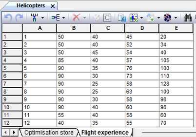
UTair's helicopter fleet operates all over the world. Special units have been created to service helicopter equipment. One of them is the aircraft repair complex of UTair Engineering JSC, which carries out major repairs, maintenance, repair and restoration work on a wide range of helicopters of various classes. In addition, the company is the leading aviation and technical base of Mi-8, Mi8MTV-1, Mi-8AMT, Mi-10, Mi-26, Mi-171 helicopters and their modifications and performs services for the delivery to and from the repair of helicopters, aggregates by any means of transport. A significant part of the helicopter fleet is operated in the regions of the North of Siberia, which, in conditions of an insufficiently developed road network, significantly increases the costs of transport logistics of spare parts and aggregates. Analysis of the distribution of the raid during the year for MI-8 helicopters (Table. 9.3) shows that the average operating time per month during the year significantly depends on the time of year, and it is determined not only by weather and climatic conditions, but also by regional operating conditions.

Table 9.3 - Distribution of the raid during the year

Calendar month


The raid in hours at the helicopter bases

Surgut

Noyabrsk

Tazovsky

Novy Urengoy

January

50

40

45

20

February

50

40

52

34

March

50

45

54

40

April

85

40

57

105

May

90

35

76

100

June's

90

30

73

110

July

90

25

58

128

August

90

25

63

100

September

90

30

58

98

October

90

40

60

98

November

55

40

58

60

December

40

35

55

70


The use of simulation modeling of the resource consumption of aggregates will allow predicting their delivery with higher accuracy and reduce logistics costs. We will build a simulation model of the delivery of the following spare parts of the MI-8 helicopter: - TV2-117 – aviation turboshaft engine, - main gearbox BP-8A, - main rotor hub HB. Losses due to the lack of replacement units, associated downtime of aircraft and storage costs in the warehouse are selected as the target function. A general algorithm for simulating the operating time of aggregates during the operation of aircraft, as well as the management of their supplies and the costs associated with this, is shown in Fig. 9.73.
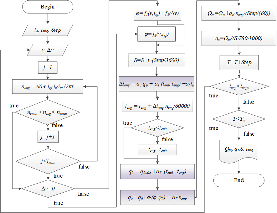
 
Fig. 9.73. Simulation model algorithm
The presented model provides the following assumptions and limitations: - operating conditions that significantly affect the reliability of helicopter components and assemblies are considered the same for the entire group of aircraft of this brand and model; - the model provides for the simulation of the operating time of units with a regulatory resource, individual components and parts, as well as their sudden failures are not simulated; - the simulation results are determined by the initial operating time of the units for each of the aircraft; - the delivery time and the availability of a serviceable unit are not simulated, but can be implemented with appropriate modification of the model. The algorithm is implemented using the "Stamm 4.2" system, the workbook sheet containing the simulation model is shown in Fig. 9.74.

 
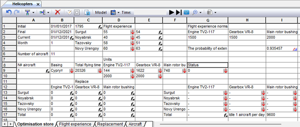
Figure 9.74. Simulation model sheet

The elements providing simulation of the consumption of the potential resource of aggregates are implemented using the built-in Stamm table processor. The model workbook also contains a worksheet that serves as a database for aircraft flight simulation (Fig. 9.75).

 
Figure 9.75. Helicopter flight simulation sheet

The elements of the simulation model created using specialized controller cells are presented in Table 9.4.

Table 9.4 - Model components created using "Stamm" controller cells

Type of controller cell

Cell or range of the sheet

Functions performed

Model time scanning

B3, C3

Determining the current calendar date based on the virtual time of the model

E2:E5

Generation of a random value of the operating time of the aircraft during the month

A9

Generating the current helicopter number

B13:D16

Modeling of replacements by units and locations

B17:D17

Calculation of the total number of replacements by aggregates for the entire simulation period

G17

Data reset at the beginning of the month  

Scanning

D2:D5

Simulation of the monthly flight of an aircraft depending on the location of the base

B9

Displaying the location of the base

C9

Simulation of the total flight of an aircraft

D9:F9

Flight on individual aircraft units

G9

The current status of the aircraft is "ready for operation", "needs replacement of the unit", "idle"


G13:I16

Modeling planned replacements by month

Random Number Generator

I5

Generating the probability of extending the life of the unit


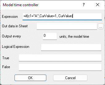
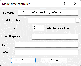
The components of the model that provide the calculation of variables, the value of which changes over the course of the model time and depends on other variables of the model, are implemented as a simple controller of the model time (Fig. 9.76).
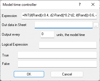
 
Fig. 9.76. The controller cell that calculates the average flight per month for this aircraft

Some model time controller cells do not perform current calculations with each change in model time, but implement logical operations, Figure 9.78 shows a cell that controls the state of the need to replace the unit. The current numerical data in the controller cell, necessary for further analysis of the simulation results, are recorded in a special sheet with a specified frequency (Fig. 9.77).

 
Fig. 9.77. The controller cell determining the moment of replacement of the unit
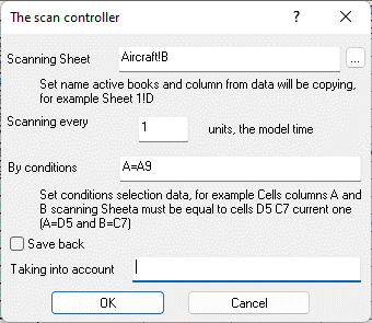
Controller cells that reproduce tabular data and functions in the model are also implemented with various settings. Reproduction in the model of the location of the current aircraft provides for a simple transfer of the tabular value of the indicator (Fig. 9.78). The scanning controller that implements the change of operating time for the TV-2-117 unit (Fig. 9.79), in addition to transferring the indicator to the model, changes its value depending on the fulfillment of the logical condition set in the controller settings and writes the new value back to the table.

 
Fig. 9.78. A controller cell that scans the aircraft data table by the "Basing" column
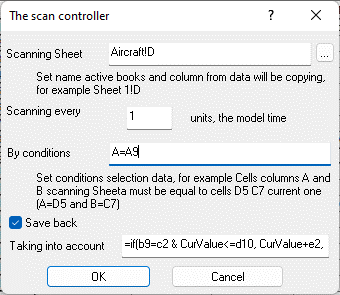
 
Fig. 9.79. The controller cell scanning the aircraft data table according to the column "Operating time TV-2-117"
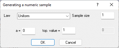
In the simulation model of unit replacement planning, only one specialized component is used, a random number generator that simulates the extension of the regulatory resource of the unit (Fig. 9.80). Nevertheless, other elements of the model contain random components. For example, a cell that simulates fluctuations in the flight time of an aircraft over a month under the influence of random factors implements this using the "Rand" function built into the table processor (see Figure 9.76).

 
Fig. 9.80. A controller cell simulating the probability of resource renewal
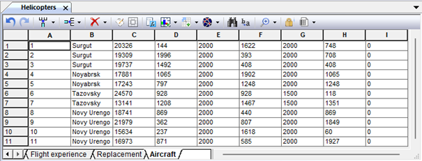
To set the initial data of the simulation experiment, the data of the sample was used, which was formed in the model itself, taking into account the available data on the age of helicopters and the flight of the units installed on them (Fig. 9.81).

 
Fig. 9.81. Initial sample of the model
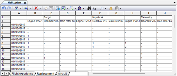
Then an experiment was conducted to simulate the operation of aircraft units and simulate their replacement. The simulation was stopped and the results were analyzed when the model time reached five years. In the process of modeling, the flight of aggregates of various types in the locations at each discrete step of the model time was calculated taking into account the calendar period reproduced in the model and regional peculiarities of changes in the intensity of aircraft operation during this period. The final raid is actually an integral quantity. Thanks to the special configuration of the model elements containing data on the flight of aggregates, a table of numerical values of these indicators obtained with a given frequency was formed (Fig. 9.82). According to the data of such tables, corresponding graphs of changes in indicators over time can be constructed.

 
Fig. 9.82. Numerical data – simulation experiment results