Introduction
The software, which has a standard interface, a simple and accessible system for organizing simulation models for unskilled users, will allow you to use the main advantage of using a personal computer - to solve an application problem right at the workplace. The initial data processing and simulation system "Stamm", which has built-in data management and modeling tools, including simulation, and has an intuitive interface similar to the popular" Microsoft Excel", does not claim to be universal, but to some extent makes the development of simulation models available to the ordinary user of personal computers (PCs). The program is created using the Stingray® "Objective Studio" and GSL libraries.Workbook
Creating a new workbook
You can create a new workbook by clicking the button on the Quick Launch toolbar or the main menu button and selecting the "Create" menu option (see Figure 1). The new workbook will consist of a single blank sheet (Figure 2). The workbook window is located in the working area of the program "Stamm" and has its own title in the form of a bookmark at the top left, all created workbooks have a bookmark of different colors. The files of the created system workbooks have the extension "swb", although later you can set any extension or delete it altogether, when you open such a file from the program, it will still be opened as a workbook. However, it is recommended to use the extension, because when you associate an application with this file type, Stamm will start automatically when you select any file with the "swb" extension in Windows Explorer. When a new workbook is created, it is named Workbook 1...N by default, where N corresponds to the number of workbooks opened during the current session with the program. Each time you start the program again, the process of setting the name of the workbook document is repeated, and when you exit the program or close the window after editing the workbook, the system asks for a unique name for it.
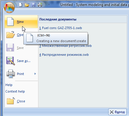
Figure 1. Creating a new "Stamm" workbook»
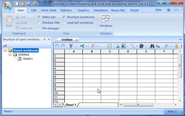
Figure 2. The new "Stamm" workbook»
Opening an existing workbook
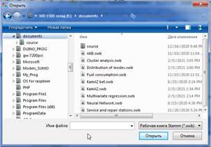
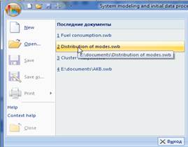
If the application is not running, you can open the workbook directly from Windows Explorer by double-clicking on the name of the desired workbook. This is possible if the file has the extension " swb "and this file type is associated with the application"Stamm" in the operating system. You can create such a link in Windows Explorer by selecting a file with the workbook extension, then open the context menu by right-clicking and selecting "Open with" – "Select program". In the dialog panel that appears, the "Use the selected program for all files of this type" property should be enabled. To complete the binding, you must select the Stamm application. From a running program, you can open the workbook by clicking the "Open" button on the Quick Launch toolbar or by clicking the main menu button and selecting the Open menu option. At the same time, the file opening dialog panel appears (Fig. 3 a). When you click the main menu button on the right, there is a list of workbooks that you previously worked with on the computer, you can select workbooks that were edited during the last 4 sessions with the PC (see Figure 3 b). The quickest way to download books to the app is through the navigation bars (see section 2.5).
|
|
| a) Through the "Open" dialog panel | b) From the list of recent books |
To save the workbook
You can save the workbook by clicking the "Save" button on the Quick Launch toolbar or by clicking the main application button and selecting the "Save" option.
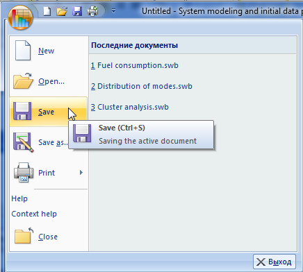
Figure 4. Saving the "Stamm" workbook»
Change the name of the workbook
You can change the name of the workbook by selecting the "Save as ..." option in the main menu (Figure 4). Another option is to use the Windows file system tools, from any file selection panel or Windows Explorer, by double-clicking on the workbook file name or pressing F2 to change it (see Figure 5).
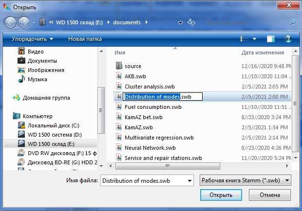
Figure 5. Changing the name of the "Stamm" workbook»
SHEETS OF THE "STAMM" WORKBOOK
The program workbook can contain four main types of sheets:- worksheet;
- simulation sheet;
- list of graphical representation of data;
- structural model sheet..
Worksheet and simulation sheet
They are spreadsheets similar to Microsoft Excel.Manipulating rows
Inserting rows
1. To insert a single row, click the cell in the row above which you want to insert a new row. For example, if you click a cell in row 2, a new row will be inserted above it. 2. In the Application Ribbon Worksheet tab, select the menu of the Row button, then the Edit-Paste option (Figure 6), or simply click the Row button.
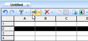
Figure 6. Inserting a line into a worksheet
Deleting rows
To delete, select the lines to be deleted on the Application Ribbon Worksheet tab, select the Line button menu, and then select Edit-Delete (Figure 7).
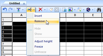
Figure 7: Deleting rows in a worksheet
Manipulation with columns
Hiding
To hide one or more columns, select them with the mouse, and then click the mouse cursor on the header of the desired column and, without releasing the left button, move the mouse until you select all the necessary columns. Then select the menu option "Format" - "Column" - "Hide". Hidden columns can be shown again in their original width by double-clicking on the right border of the column header preceding the hidden columns, or by selecting the menu option "Format" - "Column" - "Show".Insert
To insert a column, move the cursor in the table to the column before which the new one will be inserted. In the Application Ribbon Worksheet tab, select the Edit - Insert Column button menu, or simply click the Column button (Figure 8).
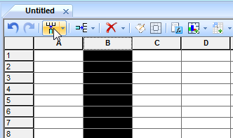
Figure 8. Inserting a column into a worksheet
Removal
You can delete any of the columns or a group of them entirely from the sheet. To do this, click the mouse cursor on the header of the desired column and, without releasing the left button, move the mouse until you select all the necessary columns. Then select the Edit-Delete option from the menu of the Column button on the Application Ribbon Worksheet tab (Figure 9).
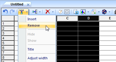
Figure 9. Deleting columns
Changing the column width
To change the width of a column, place the mouse cursor on the right border of its header (it will take the form of a bidirectional arrow) and, by clicking its left button, drag the border of the column to the desired size. To increase or decrease the size of a column, double-click on the separator line between two adjacent headers.Changing the column header
To change the column title, move the cursor in the table to the column whose title is being changed. On the worksheet tab of the Ribbon of the application, select the menu button Column Header. Or place the mouse cursor on the desired title and right-click it to select the "Title" option from the context menu. After that, you can edit the title as usual. To pin the edited title text, press the [Enter] key.Headers and footers
Headers and footers are information that is not displayed on the worksheet when working with it, but is output when the sheet is printed on the printer at the bottom (footer) and at the top (header) of the pages. You can configure the headers and footers by using the Application Ribbon option-the "Worksheet" tab-the menu of the Properties button - "Headers and Footers" (Fig. 10).

Figure 10. Calling the header and footer settings
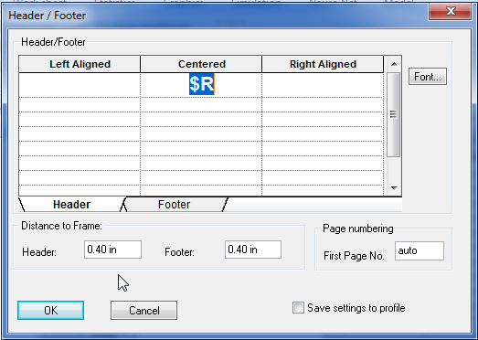
Figure 11. Setting up footers
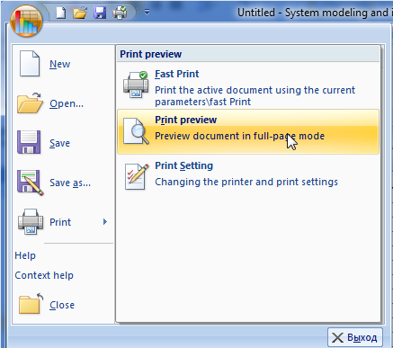
Figure. 12. Printing. Preview
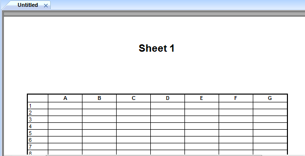
Figure 13. Preview
Search for text on a sheet
To find text on the current sheet, use the "Find" button on the edit tab of the Ribbon of the application (Fig. 14). After entering the required text in the search bar, you need to click Find next, sequentially, starting from the current cursor position, top-down will stand out matching pieces of text that are found in the cells of the sheet.
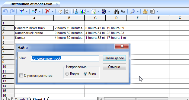
Figure 14. Searching for text in cells
General view and main elements of the graphical representation sheet
The appearance of the graphical data representation sheet depends significantly on its settings. Figure 15 shows a typical graph in the form of curves with widget points corresponding to numeric data. This type of sheet, in addition to the plot area itself, which is responsible for the graphical interpretation of the data, can contain one or more elements such as: background, captions, legends to data series, text labels and the title of the graph. All these types of elements can overlap. The plot area itself, like all other elements, is also customizable and can change the display of axes, fill, font, borders, shadows, scale, color and outline of individual points and lines of graphs, and other design.
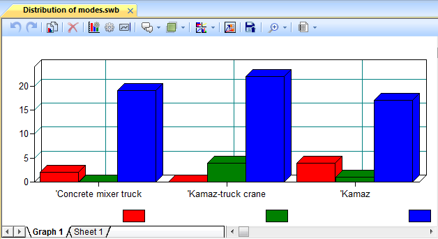
Figure 15. Sheet of graphical representation of "Stamm" data
General view and main elements of the sheet of the object model
A object model sheet is a canvas that contains typical elements that are created by the user or selected from libraries stored on the element carrier, and the model blocks can be connected by links (Figure 16). The canvas can have a grid for more precise positioning of model objects. The elements that are typed into the component model are placed within the canvas using visual design by dragging the mouse or using the keyboard cursor keys. The connection of individual components to each other is carried out using link lines, the beginning and end of which are located in ports belonging to different objects. Components connected by links behave as a whole when moving on the model canvas and rotating, changing their appearance depending on their relative position. In addition, individual elements can be grouped together for the same purpose. The properties of each element or group can be configured using a special dialog panel.
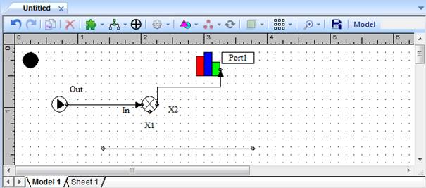
Figure 16. Sheet of the object model "Stamm"
Insert a new sheet
The Stamm workbook can contain five types of worksheets: the first is a worksheet, the second is a simulation sheet, the main difference between them is that the second option allows the organization of a simulation model of pseudo–real time (system dynamics) of a tabular type, the third type is a graphical representation of numerical data contained in the worksheet, the fourth type is combined panels containing numerical data and graphical presentations ("Distribution", "Regression", "Multivariate regression", "Cluster analysis"), the fifth type is an object simulation model and a UML structural model. The desired type is selected from the drop-down list of the "Sheet" button from the "Edit" tab of the ribbon (Fig. 17a). In addition, a similar insertion from the context menu of any worksheet is possible (Fig. 17 b). Also in the toolbar of each workbook there is a button with a drop-down menu "New", located on the left, which also involves inserting any of the possible types of worksheets (Fig. 17c).
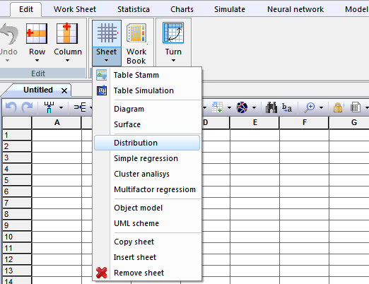
Figure 17a. Inserting, copying, and deleting a workbook sheet. Ribbon
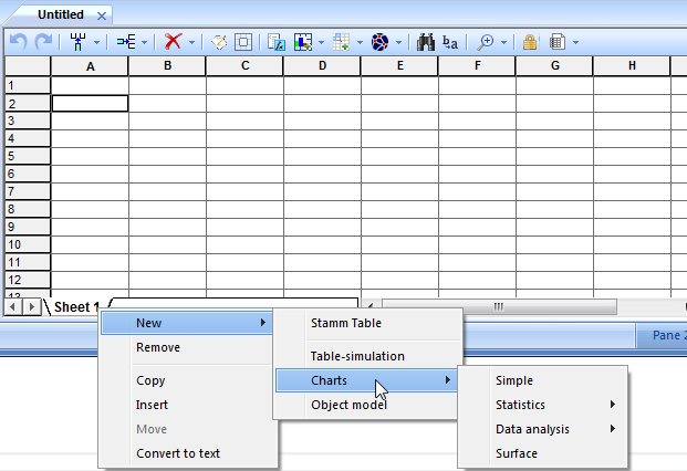
Figure 17b. Inserting, copying, and deleting a workbook sheet. The context menu of the sheet
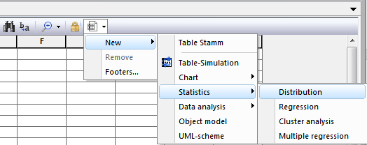
Figure 17c. Inserting, copying, and deleting a workbook sheet. Toolbar of the sheet
Deleting sheets from a workbook
Select the sheets you want to delete. To select several sheets, you need to click on their labels with the mouse while holding down the CTRL key. Select the drop-down list buttons "List" from the edit tab of the ribbon, it selects the Delete command (figure 17). Changing the display scale sheet The scale of the data display can be increased or decreased by stretching the application window out of the frame, as well as by selecting one of the options in the drop-down menu of the "Zoom" button from the "Edit" tab of the ribbon (Fig. 18).

Figure 18. Changing the scale of the data display in the workbook sheet
DATA MANAGEMENT
Numeric and other data can be stored in the work sheets of the "Stamm" workbook, the number of rows or columns in which is limited only by the amount of free memory of the system. The numbers or text in the cells can be entered from the keyboard or retrieved from the Windows Clipboard. Moreover, in the latter case, the size of the worksheet changes dynamically in accordance with the amount of data placed, for example, if the sheet contained 20 rows, and the data block placed in it contains 100 rows, then the size of the sheet automatically increases to 100 rows.Use of special cell controls
For a more convenient perception of various types of data, you can use special methods for displaying data that are available through the tab - "Controls", the "Cell" panel (Fig. 19). First, you must select the cell or range that you want to change its display type. The data display options available in the program are shown in the table. For example, data from a limited set can be represented by controls – a Drop-down list or Combo Box, and logical data in the form of a Check Box element (see Table).
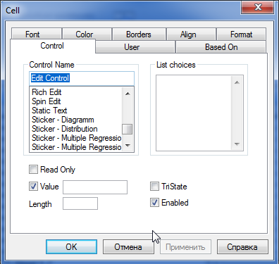
Figure 19. Cell panel
Using the formula processor
Any cell in a worksheet can contain a mathematical or logical expression that is automatically calculated when it is updated. This expression can contain both constants and variables as references to other cells. All the rules used in mathematical formulas apply to the expression in the cell, for example, the order of calculations, the use of parentheses, etc. The formula must start with the sign'=', for example, " =12.235+d1*(a1-1.2)".Built-in functions
The system's formula processor contains a set of standard functions similar to Microsoft Excel. A standard function can be entered directly into the cell from the keyboard, for example, " =AVG(12,11,22)". Another option is to use a special dialog panel containing a set of standard functions, for which we click the "Function" button on the quick launch toolbar of the book or by selecting the Edit-Function tab of the ribbon (Fig. 20).

Figure 20. The "Functions" submenu
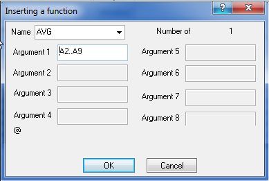
Figure 21. Standard function input panel
Data ordering
In order to sort the necessary data, select the required range of cells and right-click to open the context menu, where you can perform the sort option (Fig. 22).
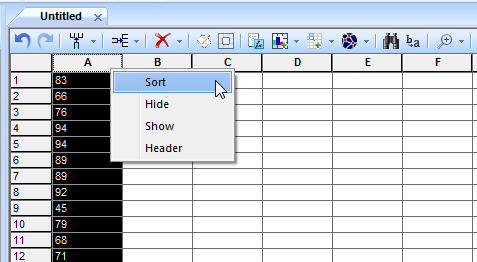
Fig. 22. Sorting numeric data
Generating random sequences
Sometimes it is necessary to obtain numerical data corresponding to a certain distribution law of a random variable with specified parameters. To do this, you need to select the cell on the worksheet from which the numeric selection will start, the data will be generated from top to bottom, starting with the selected cell. Then select the "Distribution" button from the "Statistics" tab of the ribbon (Figure 23). In the dialog panel (Fig. 24), you need to set the necessary parameters. The distribution generation is initiated by the system timer, so each new numeric sample will be unique. The distribution parameters displayed in the configuration panel change dynamically depending on the selected law. The program uses a contextual help system. In the case of generating a random variable distribution law, you can preview the probability density function used for the selected law, its parameters, the type of graph, as well as typical areas of practical use (Fig. 25).
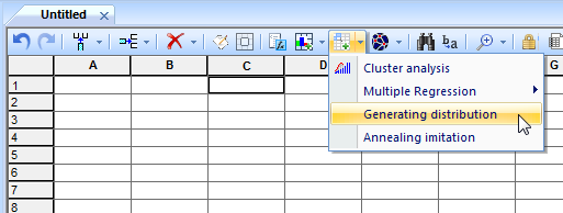
Figure 23. The statistics tab. Generating a random variable
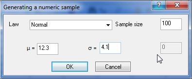
Figure 24. Generating a random number sample
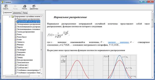
Figure 25. Contextual help
Creating and using a multi-layer neural network
At the first stage, you need to determine the location of the created neural network on the selected sheet of the program workbook. To do this, you need to select a range of cells sufficient to accommodate all the neurons in it, each of which will occupy a separate cell. After that, select the " New "option of the" Neural Network " ribbon tab in the dialog panel that appears, you need to set the name of the network, the rest of its parameters can be changed later when the network is initialized (Fig. 26).
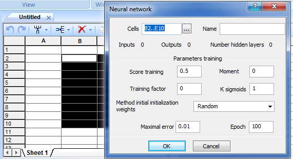
Figure 26. Creating a layout for placing the network on the worksheet
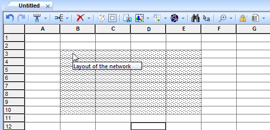
Figure 27. Layout field for placing neurons
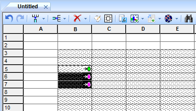
Figure 28. Creating neural network inputs
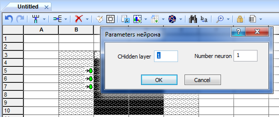
Figure 29. Creating hidden layers of neurons
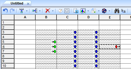
Figure 30. The creation of the outputs of the network
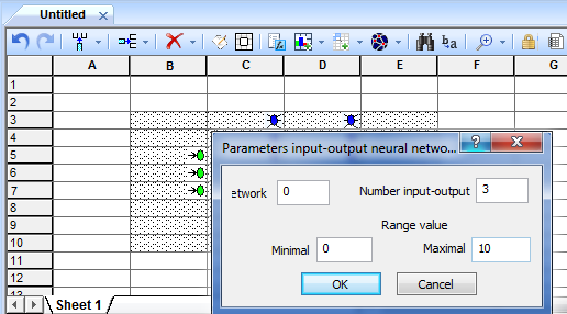
Figure 31. Tuning of neurons in the input / output
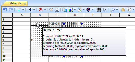
Figure 32. Initialized neural network
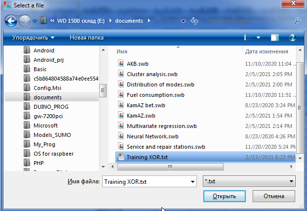
Figure 33. Selecting a file for network training
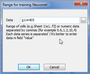
Figure 34. Selecting the data range for network training
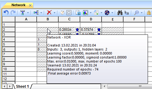
Figure 35. Characteristics of the neural network
GRAPHICAL REPRESENTATION
Numeric and other data can be stored in the work sheets of the "Stamm" workbook, the number of rows or columns in which is limited only by the amount of free memory of the system. The numbers or text in the cells can be entered from the keyboard or retrieved from the Windows Clipboard. Moreover, in the latter case, the size of the worksheet changes dynamically in accordance with the amount of data placed, for example, if the sheet contained 20 rows, and the data block placed in it contains 100 rows, then the size of the sheet automatically increases to 100 rows.Graphics-stickers
The tools of the "Stamm" system allow you to organize a graphical representation of the numeric data contained in the cells of the workbook worksheets. The special features of this representation are the vector structure of the drawings (diagrams), which, unlike raster drawings, allows you to scale the image as you like, as well as edit its individual elements. To do this, you need to select a rectangular block of sheet cells that are not occupied by data, its size should allow you to display the necessary graphs on this section, for example, a three-dimensional histogram (Fig. 36).
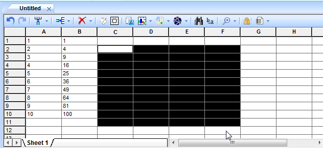
Figure 36. Selecting a range of cells for a sticker graph
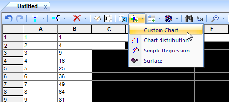
Figure 37. Inserting a sticker graph
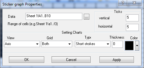
Figure 38. Chart or graph parameter settings panel
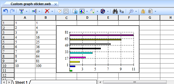
Figure 39. Graphical representation of the data range
Charts on separate sheets in the workbook
Graphics-stickers have limited options for their configuration, in contrast to them, the graphics on individual sheets of the workbook are more functional. At the same time, their creation is not at all more difficult. A graphic image sheet, like any other, is placed in the workbook to the left of the currently active one. Most variants of such graphs are created using the buttons on the Graphs tab of the application ribbon. The universal option is "Graph", which allows you to get on one sheet from one to several rows of points corresponding to numerical data in the ranges of cells with numerical data selected on the worksheets. The ranges are selected in the panel located on top of all other windows. Charts can be constructed and functional dependencies, functions must be written in the cell in the format formula CPU Stamm, adjacent cells specify the range of parameter change of the independent variable X, the last cell contains step calculations neighboring values of Y. for Example, the table below shows how a cells range from the top down in rows and from left to right across the cells to plot the theoretical curves. Table 1 № line Calculation functions of curves Point from to Intermediate 1 y=0.3851 -0.136*x + 1.292*x**2 -0.891*x**3 + 0.211*x**4 -0.0208*x**5 + 0.00073*x**6 1 10 20 2 y=sin(x) 1 10 20Inserting a graphical representation into a workbook
To insert a chart, you can use the drop-down menu of the workbook toolbar (Fig. 40) or the "Charts" tab of the "Charts" panel - "Chart". The chart settings panel appears (Fig. 41).

Fig. 40. Inserting a chart via the menu of the sheet-table toolbar
The settings panel of the graphical representation
Called when inserting a graphical representation into a workbook or from the context pop-up menu of the graph (below). It is a non-modal dialog panel that allows you to select ranges of data to display on the workbook sheets.
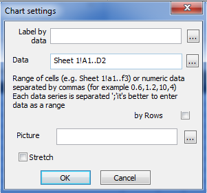
Fig. 41. The settings panel of the graphical representation
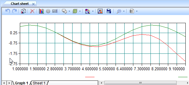
Figure 42. Graphic representation sheet
Configuring the display of graphs
The various types of graphs discussed above have common properties and functions. In the settings panel (Figure 43), graphical representations of data, as well as titles, labels, and legends, are called "Components" and have properties defined when they are created (by default). The position, background, borders, and fill can be changed by the user when selecting this component from the list, for example, by double-clicking the mouse. The graph elements associated with the data can also be configured individually through their properties settings panel, which is called when the corresponding element is selected from the list.
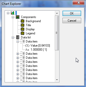
Figure 43. Chart Settings panel-Explorer
The position of the component
Each component has rectangular coordinates. The settings panel can position the component in one of four measurement modes: pixel, metric (millimeters), inches, and percentages (Figure 44).
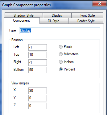
Figure 44. The Graph settings panel. The position of the component
The appearance of the borders of the component, its background and shadow are controlled using the settings panel on the corresponding tabs (Fig. 45 - 47).
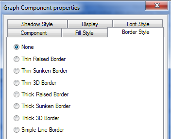
Figure 45. Chart settings panel. The bounds of the component
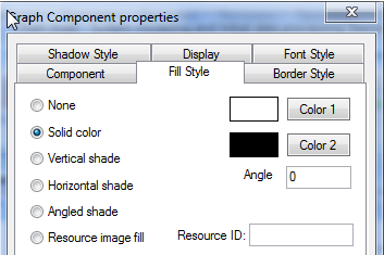
Figure 46. Chart settings panel. Component Fill Styles
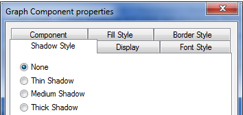
Figure 47. Chart settings panel. Styles of the shadow component
The appearance of the component itself is controlled using the settings panel on the build area tab (Figure 48).
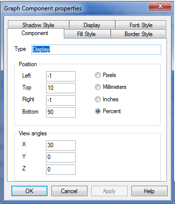
Figure 48. Chart settings panel. Plot area
The individual component elements associated with the data are controlled using their own settings panel (Figure 49).
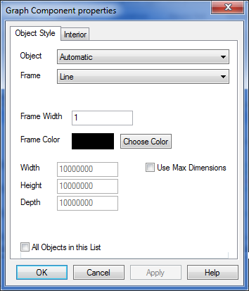
Figure 49. Settings panel for graph elements related to data
Relationship between data and graphical representation
Creating a chart on a separate sheet in the workbookTo embed a sheet with a graphical representation of the data, you must:
- select a sheet with the necessary data in the workbook,
- select a range of data to display,
- select the desired type of graphical representation from the "Graphs" tab of the application ribbon.
At the same time, a graphical representation sheet is created and embedded in the workbook, to the left of the data sheet, and its properties can be configured individually through the "Properties" and "Settings" panels. Configuring data communication
The mode of graphical display of data can be changed via the Properties panel, the appearance of this panel depends on the type of graph specified when creating it (Fig. 41, 50, 51). This window allows you to change the range of displayed data, and it does not capture the focus, that is, it allows you to go to any of the sheets of the workbook to select a range of cells.
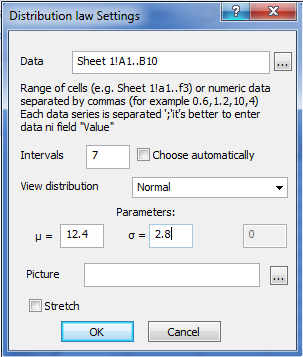
Figure 50. Chart data settings panel
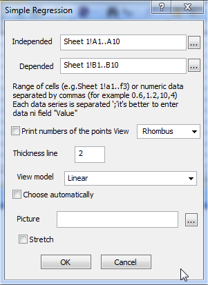
Figure 51. Simple regression data configuration panel
In the mode of graphical display of numerical data, the vertices of the graph can be changed by dragging the corresponding point or line, the changed value of the Y coordinate can be synchronized with the numerical data of the corresponding point in the data sheet specified in the graph properties. This function is called by clicking the "Sync" button in the "Charts" panel of the ribbon. When you change the numeric data in the sheet itself, the corresponding graph changes automatically. When you delete a sheet with numeric data from the workbook, the graphical representation "forgets" about the relationship with the data, however, the graph remains as it was up to this point. And its data can be changed through the "Settings" panel or manually.
Editing graphical views of a workbook
Graphics Explorer
The graphical representation of numerical data (diagrams, approximations, frequency histograms, etc.) created in "Stamm" can be customized to meet the preferences and tastes of the user. To edit individual elements on a graphic representation sheet, use visual editing technology - drag-and-drop with the mouse, component context menus, or the graph explorer. The graph explorer is a dialog panel that contains a structured list of all the elements of the current graph view sheet (Figure 52). The properties of any of the graph elements are configured using contextual dialog panels that are called when the left mouse button is double-clicked on the selected component. Also, any of the elements can be created, moved or deleted using the context menu of the explorer, which is called when you right-click on any of the elements.
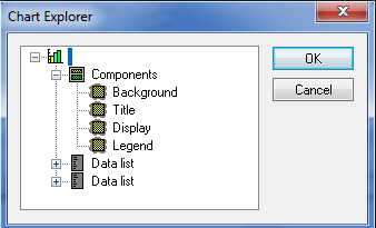
Figure 52. Explorer of the graphical representation
Components of the graphical representation of data
Types of chart componentsThe components that form the appearance of a graphical data representation sheet include: - plot area (fig. 53) below the chart title;
- chart title (fig. 53) at the top;
- axis labels of the graph (fig. 53) at the left;
- legend (fig. 53) grey box;
- text panels (fig. 53) box with border and shadow.
Each component performs its own function, its position, size, and properties can be changed through the editing panel, accessible by selecting the "Properties" option in the context menu, which is called when the right mouse button is pressed when the cursor is on the component field. The main component of the graphical presentation, the only one considered that should always be present on this type of sheet is a plot (Fig. 53).
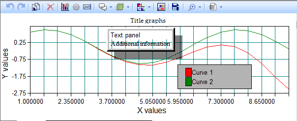
Fig. 53. The components of the graphical representation

Figure 54. The context menu of the "Legend" component»
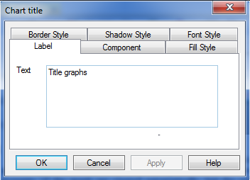
Figure 55. The panel for editing the properties of the component "Title"
Creating components
When creating a new graphical representation of numerical data (diagrams, approximations, frequency histograms, etc.), the necessary components of the graph are created automatically, but the additional components specified above can be placed on the field of the visual representation sheet for explanations of graphs, axes, text notes, etc. There are three ways to create new components on the graphical view: create a new component via the context menu or the Graphics explorer, insert a copy of an existing component using the Windows Clipboard, or load a copy of it from a template previously saved on the media. To insert a new component in the graphical representation with the help of the context menu, you must place the mouse cursor on a free from other components of the chart and press the right mouse button in the appeared context menu select submenu Components from which to select the type of the component (Fig. 56). In this case, the dialog panel for configuring the properties of the new component will immediately appear (Fig. 55). To create a component from the graphical view explorer, you need to open it by double-clicking the left mouse button when the cursor is on the graph field. Select the "Components" branch, and then right-click to open the explorer context menu (Figure 57). In this menu, select "Add Component". In the "Select Component" dialog panel, open the drop-down list and select the desired type (Figure 58).
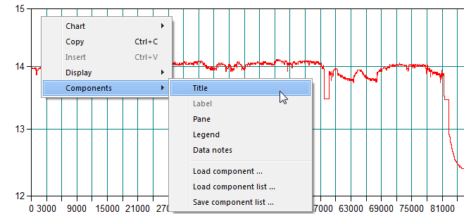
Figure 56. Creating a new component of the graphical representation
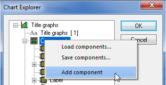
Figure 57. Creating a new component of the graphical representation via the explorer
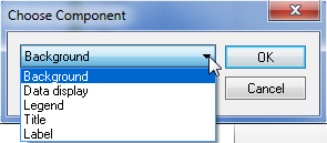
Figure 58. Creating a new graphical representation component via the explorer
The movement of the components of graphical representations
Any of the above components of the graphical representation of data can be moved within the graph field. To do this, click the left mouse button when its cursor is on the desired component and, without releasing it, move it to the desired place on the chart, then release the button. In this case, the new position of the graph element on the screen can be observed using a special cursor and a rectangle that matches the size of the object being dragged (Fig. 59).

Figure 59. Moving the component
Resizing
The size of the rectangle occupied by the graph component on the screen can be changed by the user. To do this, place the mouse cursor on the border of the object, left, right, top or bottom, until it turns from an arrow pointer to a resizing cursor (Figure 60). After that, by pressing the left mouse button and not releasing it, you can stretch the border of the component to the required size, then release the button. In this case, the future position of the borders of the graph component on the screen can be observed using a rectangle (Figure 60).
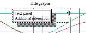
Figure 60. Resizing the component
Copying components
To create a copy of the components, use the clipboard or templates that are uploaded to the media. To create copies of any graph element using the Windows clipboard you must place the mouse cursor on the selected object and click the right mouse button, in the pop-up context menu select the item "Copy" (Fig. 61). Then move the pointer to the location of the chart or place on a different graphical representation in any open workbook and again right-click, now you must select from the menu the option "Paste" (Fig. 62). You can also paste a copy of the component from the clipboard and through the "Paste" button of the "Home" tab of the application ribbon. In this case, you cannot insert a copy of the component if it overlaps another object-a component of the graph, the cursor must be placed on an empty field of the graph.
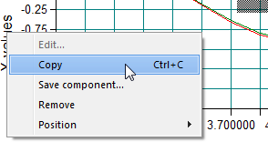
Figure 61. Copying a component
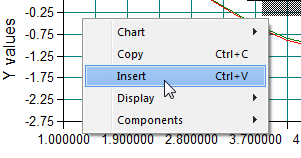
Figure 62. Inserting a copy of the component
Deleting a component
To delete components, place the mouse cursor on the selected object and click the right mouse button, select the "Delete" option in the pop-up context menu that appears (Fig. 63).
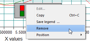
Figure 63. Deleting a component
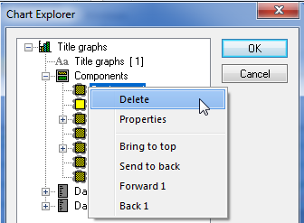
Figure 64. Deleting a component via the explorer
The position of the components
The visibility of individual graph components is determined by their position relative to other objects. If a component is behind another one, and its coordinates are within the last one, then it will be invisible on the screen. To change the relative position of the graph elements, you can use the component's context menu. To do this, place the mouse cursor on the selected object and click the right mouse button, in the pop-up context menu that appears, select the "Position" submenu (Fig. 65), in which you select the desired position of the component relative to the others. There are possible options here – place the component in the foreground, behind all the others, or move it one position back or forward.
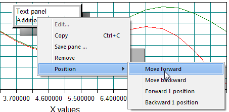
Figure 65. Component position menu
Chart Data
The data used to build graphical dependencies is stored together with the graphical representation in its properties and can be changed directly in the corresponding worksheet of the workbook. Numeric data can be grouped, for example, if several lines are drawn on a single graph sheet, then the numeric data for each of them belongs to a separate group. Data groups can be edited via the graphical representation explorer (Figure 66).The group can have a text note (see section).
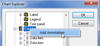
Figure 66. Changing data groups via the explorer
As noted above, changing numeric data is possible through the graphical representation explorer. To do this, after calling the explorer, you need to select the desired data group, called the "Data List", and then select the necessary element. In each data element, two fields are available for editing, one is the numeric variable itself, the other is a text note to the data element (Figure 67). After double-clicking on the desired option, it is available for editing (Figure 68).
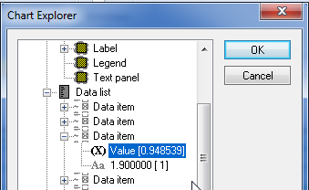
Figure 67. Editing data via the explorer
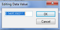
Figure 68. Changing numeric data
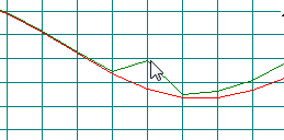
Figure 69. Editing data by dragging vertexes
Text notes for data groups are required, for example, when displaying a legend. To create or edit text notes, place the mouse cursor on a field that is free of components and open the graph context menu, where you can select the "Components" - "Data Notes"submenu option. At the same time, you must enter the desired text in the bookmarks of the editing panel (Figure 70). The number of bookmarks in the panel (Figure 71) will depend on the number of data series used in the plotting area.
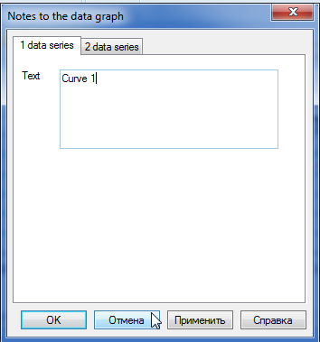
Figure 70. Editing text notes to data

Figure 71. Creating the text of the data note
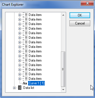
Figure 72. Changing the text of the data note
Using graphs outside of the program
The graphical representation of numerical data (diagrams, approximations, frequency histograms, etc.) created in "Stamm" can be used outside the system, since it has the Windows Extended metafile (EMF) format – the standard vector graphic format of this operating system. When transferring images to other applications, it is recommended to use this format, since the vector image retains all its qualities when zooming, there is no pixelation, loss of sharpness and font distortion. And in addition, the image itself imported in this form can be edited by almost all applications that support EMF, for example, MS Word. You can change the colors of lines and fill shapes, and select caption fonts. Change the relative position and size of individual primitives, group and ungroup them. For correct insertion in the metafile format, it is recommended to use the "Special Insert" -"Metafile" option in a third-party application. There are two ways to use graphs in other applications: the first is to use the Windows Clipboard, and the second is to save the drawing to a separate file. To copy an item to the clipboard, right - click on the main field of the graph, away from the components, and select "Copy" from the context menu (Fig. 73).
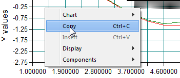
Fig. 73. Copying the graph to the clipboard
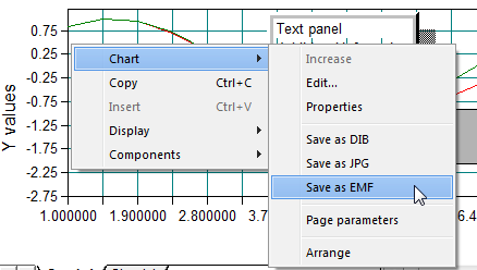
Figure 74. Writing a graph to a metafile
Format " JPG " (Joint Photographic Experts Group) it is a compressed format that significantly reduces the size of the destination file. However, if the background of the graph is white or transparent and the graph itself is a line, then using "JPG" can lead to noticeable artifacts on the borders of the grid and the graph. At the same time, the use of this format is justified when using the fill and the background of the graph in the form of a drawing.
The "EMF" (Microsoft Enhanced Metafile) format is an updated version of the WMF format. The metafile itself, unlike "DIB" and "JPG", is a vector image format, which significantly reduces the size of the destination file. In addition, a drawing saved in the "EMF" format takes up on average half as much space as the corresponding WMF file.
NUMERICAL DATA ANALYSIS "STAMM"
To analyze the data, you can use the statistical functions contained in the formula processor of the" Stamm "system, by clicking the" Function " button on the Worksheet tab of the application ribbon. In addition, the system implements a number of the most common data manipulations, presented below.The law of distribution of a random variable
In all cases of interpretation of numerical data-sample characteristics, regression dependencies, graphs, diagrams, etc., either a graphical representation or a sticker cell is used.The histogram and the theoretical distribution curve in the cell-sticker
If you use a sticker cell on the worksheet to interpret numeric data, you must first select the range of cells of the required size (Section) in which the results will be located (Figure 75). If you do not mark the cells, the sticker graph will have a standard size, by default-5 columns by 15 rows, and the upper-left corner of the view rectangle will be in the current cell.
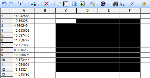
Figure 75. Preparing the data interpretation area
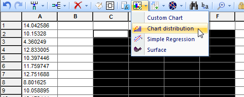
Figure 76. Statistics menu tab
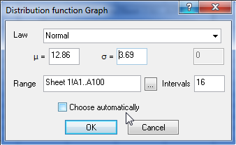
Figure 77. Distribution parameters input panel
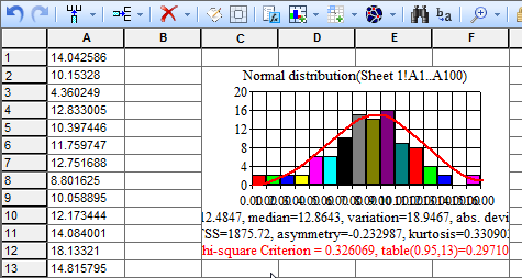
Figure 78. Visual evaluation of the distribution law
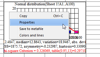
Figure 79. Context menu graphics-stickers
Histogram of the distribution on a separate sheet of the workbook
If you use this option, select the "Distribution" option in the "Statistics" panel of the "Charts" tab of the application ribbon or the drop-down menu of the "Sheet" button on the grid sheet toolbar.In the dialog panel that appears, select the distribution type and specify the range of cells that contain the digital data to be interpreted (Figure 80). The panel is non-modal, i.e. it is located on top of all other application windows and does not capture the input focus. Therefore, to enter a range of cells, you can set the cursor in the "Data" field of the panel and then move the focus to any worksheet and select the range by dragging the mouse cursor while the left button is pressed, the characteristics of the selected range are automatically transferred to the panel (Figure 80).
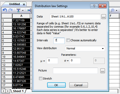
Figure 80. Data block for estimating the distribution law
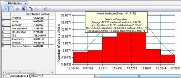
Figure 83. Visual evaluation of the distribution law
Getting regression dependencies
Getting a one-factor regression
The program "Stamm" allows you to determine the numerical values of the parameters of the pair regression equation and build an approximation line. In this case, it is possible to graphically interpret the data with an approximating curve either on a separate sheet of the workbook, or on a sticker graph and on the same sheet where the interpreted data is located.Getting a one-factor regression on a data worksheet
For this option, you need to select a rectangular block of sheet cells that are not occupied by data, its size should allow you to display a graph of the regression line and its parameters on this section (Fig. 84). After selecting the option of the "Worksheet" "Thumbnails" "Simple Regression" ribbon tab or the drop-down menu of the "Controls" button on the grid sheet toolbar (see Figure 85), a panel will appear for setting the regression parameters selected by the experimenter (Figure 86).
By selecting the type of regression equation, you must specify the range of cells that contain the independent (explanatory-predictor) and dependent (explicable) variables. This can be done from the keyboard, but it is better to use another option. The panel (Fig. 86) is non-modal, that is, it is located on top of all other application windows and does not capture the input focus. So to enter the range of cells you can set the cursor in the "Independent variable X" panels, or "Dependent variable Y", and then move the focus to any worksheet and highlight the range, holding the mouse cursor while pressing the left button, the characteristics of the allocated range is automatically transferred to the panel (Fig. 86).
After selecting all the parameters, you can press the OK button panel to output the results of the regression analysis.
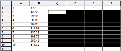
Figure 84. Marking the field for the "Simple Regression" sticker graph

Figure 85. Inserting the "Simple Regression" sticker graph
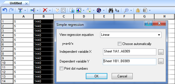
Figure 86. Dialog panel for setting regression analysis parameters
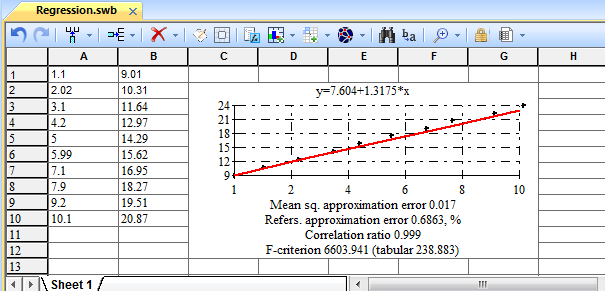
Figure 87. Regression analysis results sheet
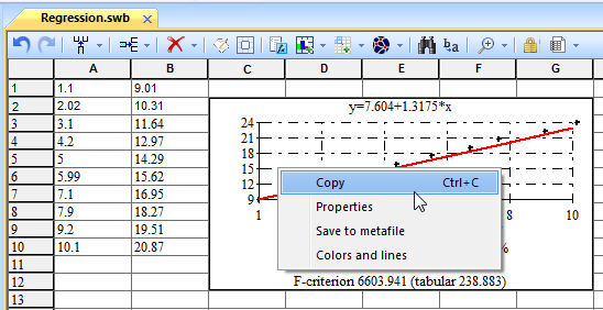
Figure 88. Context menu of the "Simple regression" element»
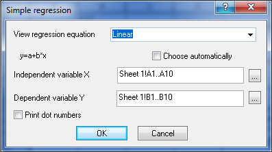
Figure 89. Panel to configure the properties of the approximating line regression analysis
Getting a single-factor regression on a separate sheet
First, in one of the worksheets, we will prepare the source data in the form of pairwise series of points, and the independent and dependent variables can be arranged as you like, although this can also be done during the setting of the regression parameters in the next step.To get a graphical representation of the data approximation on a separate sheet, use the "Regression" option of the "Statistics" panel of the "Graphs" tab of the application ribbon or the menu of the "Sheet" button of the book toolbar (see Figure 90). In the dialog panel that appears (Figure 90), enter the necessary parameters. To specify ranges of numeric data, we use the fact that the parameter settings panel is a non-modal window, that is, it is always in the foreground and does not capture the input focus. This means that by placing the cursor in the "Independent" or "Dependent" field of the panel, we can move it to any worksheet with numeric data and select the desired range of numeric data there by dragging the mouse cursor with the left button pressed. Information about the selected data block is automatically placed in the corresponding field of the panel (Figure 90).
After clicking the " OK " button in the parameter settings panel, a sheet will appear with the interpretation of the initial data for the first regression variant – linear dependence (Fig. 91). The default sheet name is "Regression N", where N is the number of sheets with graphical interpretation of the data in the active workbook.
Choose the type of regression equation and specify the range of cells in which there are independent (explaining the predictor) and dependent (dependent) variables, you can click the "Properties" panel "Appearance" tab "Charts" tape app, or via the context menu of the graph (Fig. 92), this will open the editing panel properties (Fig. 90).
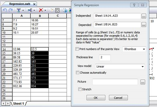
Figure 90. Call of the panel of the dialog to define parameters of a regression analysis
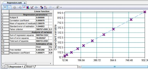
Figure 91. Interpretation of the regression analysis of data
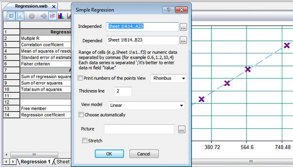
Figure 92. Changing the parameters of the regression analysis on the representation sheet
Obtaining a multivariate regression dependence
The program "Stamm" allows you to determine the numerical values of the parameters of the multivariate regression equation. To do this, you can select a rectangular block of cells on the sheet or place the cursor in a cell that has enough free space to the right and bottom of it, and the dimensions of the multi-factor regression sticker will be determined automatically. Next, select from the drop-down menu of the "Regression" button of the "Statistics" tab of the application ribbon one of the options "Multivariate OLS" or "Levenberg-Marquardt multivariate" (Fig. 93) or the drop-down menu of the "Controls" button on the grid sheet toolbar similar to the ribbon panel.
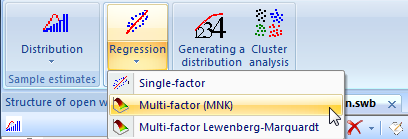
Figure 93. Calling the panel of multivariate regression analysis
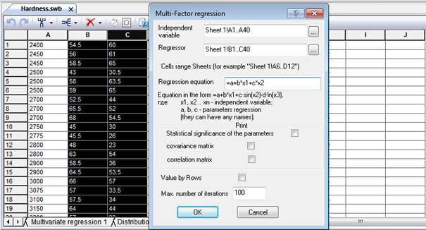
Figure 94. The panel for configuring the properties of multivariate regression analysis
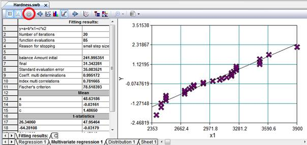
Fig. 95. Sheet multivariate regression analysis, least squares
The manipulation of data to multivariate regression
Configuring Properties
The properties of multivariate regression analysis are edited in the dialog panel discussed above (Fig. 94), which is accessible via the Properties button of the worksheet toolbar, highlighted with a red circle (Fig. 95). After evaluating the output results, you can adjust the type of equation or its parameters and re-run the least squares regression analysis procedure. Copying an item
You can copy the multi-factor regression analysis panel via the Copy context menu option (Fig. 96) or by selecting the Home tab button in the application ribbon, and you can also use the keyboard shortcut "Ctrl+C". The result depends on which of the windows of the "Multifactor Regression" sheet is active, if these are numerical approximation results, then text data will be in the clipboard, otherwise the current graphic image.
If text data and a third-party application are used for copying, then pasting from the buffer puts regression parameters there in text format, and tab characters are used as separators, which makes it possible to use them, for example, in Microsoft Excel without additional editing (Figure 98).
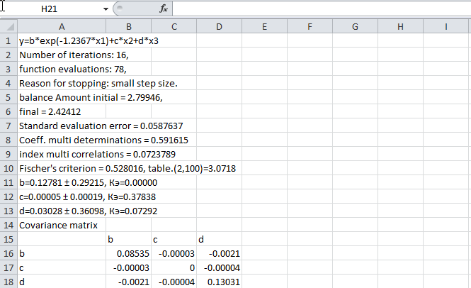
Figure 98. Inserting regression analysis parameters in Microsoft Excel
When selecting the left panel - "Graphs" of the "Multivariate Regression" control, the buttons for controlling the graphical interpretation of data are available, the desired type of graph is selected by the switch buttons highlighted in Fig. 99 with a red rectangle. For example, the graphs of the spread of parameters are multiples of their number in the regression dependence, which can be scrolled with arrow buttons (Fig. 99). These graphs allow you to visually assess the nature of the spread of parameters and the influence of each of the factors on the resulting variable.
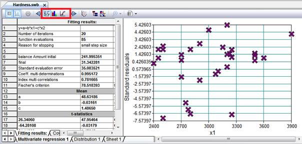
Figure 99. Graphical representation of regression analysis parameters
Spectral data analysis
Fourier transform
The Fourier transform was originally conceived as a universal method for the mathematical description of thermodynamic processes. In the future, it became widely used in the processing of modulated electrical signals. In signal processing and related domains, the Fourier transform is usually considered as the decomposition of a signal into frequencies and amplitudes, that is, a reversible transition from time space (time domain) to frequency space (frequency domain). Currently, the method has gained a second life and is used in many fields of science - in physics, number theory, combinatorics, signal processing, probability theory, statistics, cryptography, acoustics, oceanology, optics, geometry, and many others [1]. The rich application possibilities are based on several useful properties of the transformation:- Transformations are linear operators and, with appropriate normalization, unitary (a property known as Parseval's theorem, or, more generally, as Plancherel's theorem, or, more generally, as Pontryagin's dualism).
- The transformations are reversible, and the inverse transformation has almost the same form as the forward transformation.
- Sinusoidal basis functions (or rather, complex exponents) are eigenfunctions of differentiation, which means that this representation turns linear differential equations with constant coefficients into ordinary algebraic ones (For example, in a linear stationary system, the frequency is a conservative value, so the behavior of the function at each frequency can be solved independently).
By the convolution theorem, the Fourier transform turns a complex convolution operation into a simple multiplication, meaning that they provide an efficient way of computing based on convolution operations such as multiplying polynomials and multiplying large numbers.
The discrete version of the Fourier transform can be quickly calculated on computers using the Fast Fourier Transform (FFT) algorithm. A similar algorithm is implemented in the program "Stamm" 3.0.
To determine the parameters of the Fourier transform and visually evaluate its quality, just select the "Fourier" button on the "Spectral Analysis" panel of the "Graphs" tab of the application ribbon. After that, the panel for configuring the properties of the Fourier transform will appear (Figure 100). This panel is non-modal, which makes it much easier to enter cell ranges with numeric data for analysis, similar to selecting links to cell blocks for charts and formulas in MS Excel. The properties of non-modal panels are discussed in the previous sections.
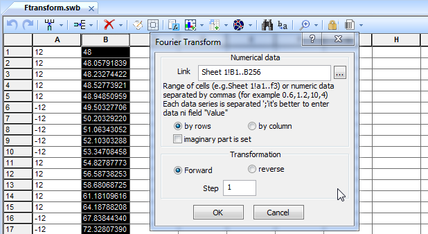
Figure 100. Configuring the parameters of the Fourier transform
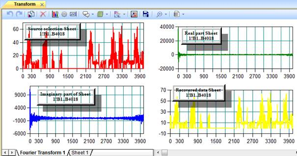
Figure 101. Inserting a sheet of a graphical representation of the Fourier transform
The conversion settings can then be set using the context menu option "Properties" sheet graphical representation (Fig. 102) or clicking the "Properties" panel "Appearance" tab "Charts" application ribbon.
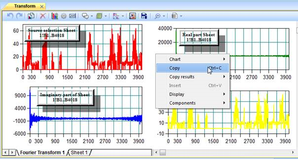
Figure 102. Context menu of the Fourier transform
Wavelet transform
The wavelet transform from the English wavelet - a small wave, ripple or waves following each other, in contrast to the Fourier transform, has become widespread relatively recently. Wavelets are a family of functions that are local in time and frequency ("small"), and in which all functions are derived from one by means of its shifts and extensions along the time axis (so that they "follow each other").The development of wavelet analysis began with the work of Haar in the early twentieth century. The theory was most developed at the end of the twentieth century, mainly due to the need for technologies for compressing and processing digital images and sound.
The program "Stamm" 4.0 uses the functions of wavelet analysis. To perform the conversion of numerical data, select the "Wavelet" button in the "Spectral Analysis" panel on the "Graphs" tab of the application ribbon. After that, the panel for configuring the properties of the wavelet transform will appear (Fig. 103). A distinctive feature of this panel is the setting of the connection between the user-selected range of cells in randomly selected worksheets of the Stamm workbook and the Data input field, similar to the selection of links to cell blocks for charts and formulas in MS Excel. The panel itself always remains visible.
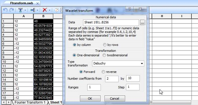
Figure 103. Configuring the parameters of the wavelet transform
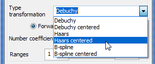
Fig. 104. Configuring the parameters of the wavelet transform
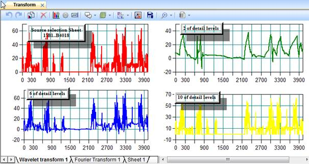
Fig. 105. Visual representation of the wavelet transform
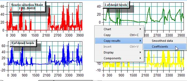
Fig. 106. The context menu of the wavelet transform
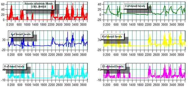
Figure 107. Visual representation of the wavelet transform
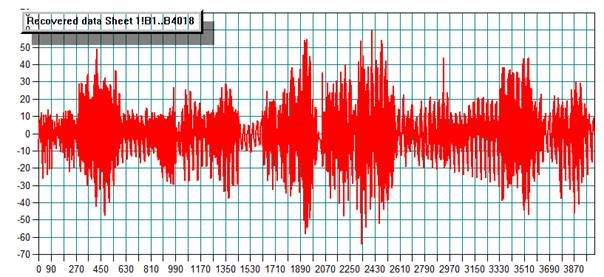
Figure 108. Visual representation of the inverse wavelet transform
Cluster analysis
Purpose and scope of use
Cluster analysis is a statistical procedure for processing multidimensional data in order to obtain relatively homogeneous groups. Most researchers are inclined to believe that for the first time the term "cluster analysis" was proposed by the mathematician R. Tryon. The application areas of cluster analysis are diverse, and data clustering is widely used in various branches of science and technology.Cluster analysis performs the following main tasks:
- Development of a typology or classification.
- Research of useful conceptual schemes for grouping objects.
- Generating hypotheses based on data analysis.
– Hypothesis testing or research to determine whether the types (groups) identified in one way or another are actually present in the available data.
Regardless of the subject of study, the application of cluster analysis involves the following steps:
- Selection of the sample for clustering. Usually quantitative data is used, but in the case of using a different type, it must be encoded in numbers.
- Definition of the set of variables by which the objects in the sample will be evaluated, that is, the feature space.
- Calculating the values of a measure of similarity (or difference) between objects.
- Using the cluster analysis method to create groups of similar objects.
– Checking the validity of the results of the cluster solution.
Preparing the source data
The original selection is placed on the data sheet in any place, you only need to place the data sets line by line under each other. In this case, the columns of the data range will correspond to the individual characteristics of the multidimensional selection. In the first line, it is convenient to place the name of the features (Fig. 109).
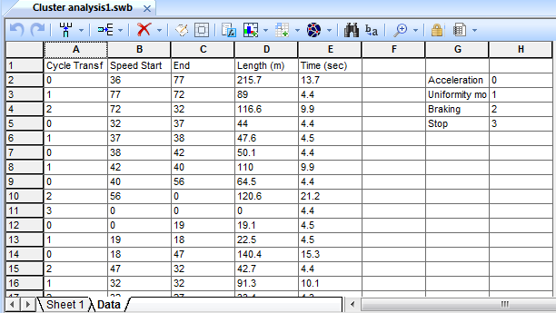
Figure 109. Source data for cluster analysis
Creating a "Cluster Analysis" worksheet
After preparing a multidimensional sample, a "Cluster Analysis" sheet is placed in an arbitrary place in the workbook, for which the "Cluster Analysis" option of the "New Sheet" button drop–down menu of the workbook toolbar is used (Fig. 17с).In the dialog panel that appears, specify the range of cells with previously prepared data for clustering (Figure 110) and select the necessary parameters.
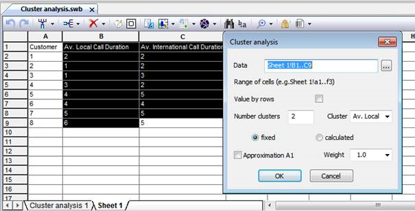
Figure 110. Settings Panel
After confirm the settings by pressing "OK" on the dialog box on the worksheet displays control "Cluster analysis", which change dynamically depending on the settings (Fig. 111). The analysis parameters and the selection can be changed using the context menu opened by right-click.
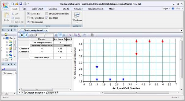
Figure 111. The "Cluster Analysis" control»
SIMULATION MODELS OF THE TABULAR TYPE
Principles of creating a simulation model
The main function of the "Stamm" system is to create simulation models of complex processes and systems that cannot be analytically described.Simulation (situational) modeling is a method that allows you to build models that describe the processes as they would take place in reality. Such a model can be "played" in time for both a single test and a given set of them. In this case, the results will be determined by the random nature of the processes. Based on this data, you can get fairly stable statistics.
When solving engineering problems on a PC, simulation is often carried out by the Monte Carlo method.
At the moment, there are three main types of simulation modeling-a relatively new direction-agent modeling, which is used to study decentralized systems, the most common discrete-event modeling, and system dynamics, where a PC reproduces a model created on the basis of graphical diagrams of causal relationships and global influences between the elements of the system under study.
In practice, quite often there is a case when, strictly speaking, the process is not random, however, its analytical description is difficult, for example, the change in time of the speed of the car when driving along the urban driving cycle obtained by field tests (Athens, New York driving cycles). Instead of using an analytical description of the process of changing the speed over time, you can reproduce the curve of this process in model time. In this case, the speed profile is set by discrete samples. This approach is implemented when creating simulation models in the "Stamm" system. For this purpose, a special control body is used - the controller, which selects the values of the variable from the profile database, according to the current value of the model time.
In addition, in nature, as a rule, if some physical objects have an effect on others, then the opposite effect also takes place. Every action provokes a reaction. Computer models are the best way to reproduce this interaction. However, systems like Microsoft Excel cannot specify the interaction of objects in the form of mathematical formulas, since they do not allow cross-references between cells. A distinctive feature of the "Stamm" simulation subsystem is the ability to mathematically describe the interactions of objects using cross-references. The second special control body is a controller that can perform calculations based on the specified dependencies, taking into account cross-references, the accumulated value of the variable, the model time and the simulation step.
Since the simulation subsystem "Stamm" is created on the basis of a multidimensional spreadsheet, similar to Microsoft Excel, these two types of controller are implemented in the form of table sheet cells with special properties. In addition, a formula processor built into the system is used to organize mathematical and logical dependencies.
Inserting a simulation model sheet into the workbook
For the development, debugging and operation of simulation models, a special sheet of the "Stamm" workbook is intended - "Simulation Sheet". It contains cell controllers that allow you to organize the simulation model, and in addition, it has additional functions for configuring and managing the simulation process. In order to place a simulation sheet in the workbook, select the "Simulation Model" option from the drop-down menu of the "Sheet" button on the "Insert" panel of the "Edit"application ribbon tab.Installation and setup of the cells controllers
All cells of the "Simulation" sheet can participate in the simulation model process, thanks to the ability to write formulas, numeric values, and references to other cells there. The key role in the simulation process is played by special cells-controllers, which can only be used in the simulation model.In order to create these controller elements in the simulation model sheet, you need to use the "Simulation" ribbon tab, then place the cursor in the desired cell and click the "Properties" button in the "Controllers" panel (Figure 112), or use the similar drop-down menu of the "Controllers" button on the sheet toolbar (Figure 113), and finally select the desired controller type from the menu . To further configure or edit the properties of the controllers, simply click the "Properties" button, or double-click the left mouse button when its cursor is located on the controller cell.
All controller cells are processed by the system when the model is started, and the numeric values stored in them can be used throughout the entire time the workbook is opened by other cells or, for example, by graphical representations of data.
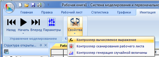
Figure 112. Creating a "Stamm" controller cell using the ribbon

Figure 113. Creating a "Stamm" controller cell using the Sheet toolbar
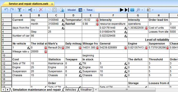
Fig.114. Selecting the controller cells on the sheet
The first one, which recalculates the parameters of the car with a change in the model time according to special dependencies set in the properties of this element, is called the "Model Time Controller". A formula that reflects the dependency simulated by the controller may contain references to other cells in the sheet (Figure 114). In this formula, you can use all the types of functions supported by the system's formula processor, listed above.
Unlike formulas in normal sheet cells, an expression in the model time controller can contain special variables – the current model time ( CurTime), the modeling step (Step), and the current value of the numeric variable in this cell (CurValue), calculated at the previous step of the model operation.
All controller control panels are non-modal windows (see above) and involve entering references to cell ranges without using the keyboard using the mouse manipulator.
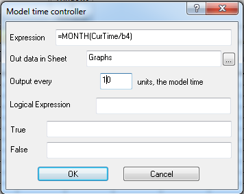
Figure 115. Properties of the "Calculated expression" controller»
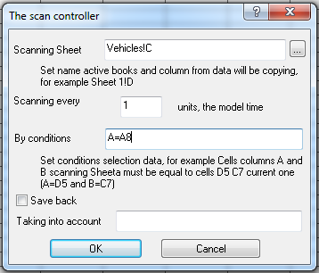
Fig. 116. Controller properties "Scan"
The third type of special cell-generating a random numeric variable corresponding to the distribution law specified in its properties with certain parameters, is called a "Random Variable Generator" (Fig. 117).
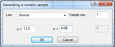
Figure 117. Properties of the "Random Variable generation" controller»
Simulation Management
In order to configure the simulation model execution modes, you need to select the "Parameters" button on the "Simulation" tab of the application ribbon in the "Simulation Management" panel (Figure 118) . In the window that appears, the panels (Fig. 119) it is necessary to set the value of the current model time to the minimum value or zero. If you need to complete the simulation by condition, for example, to reach a numeric variable in some cell of the specified value, you must put the appropriate mark.To start the simulation, click the "Simulation" button on the "Manage Simulation" panel. The simulation ends automatically when the model time reaches the limit value set in the settings panel or when the condition set in the simulation parameters is met (Figure 119). You can pause the simulation model by clicking the "Pause" option from the "Simulation" drop-down list (Figure 11). The simulation will continue when the model is run again as indicated above.
Sometimes, to debug the model, you can perform a step-by-step simulation, using the "Forward one step" and "Back one step" buttons. In this case, the model time increases or decreases by the value of the simulation step set in the settings panel (Figure 120), all relationships are recalculated, and the simulation is stopped.
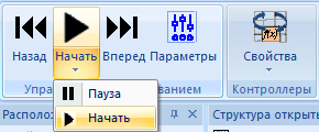
Fig. 118. Simulation model control menu ribbon
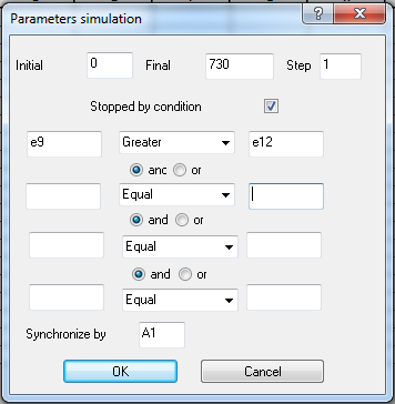
Fig. 119. Simulation model control buttons toolbar sheets
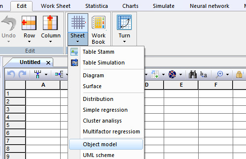
Figure 120. Panel set the parameters of the simulation model
Creating system dynamics models
Most of the examples of models discussed in this book belong to the class of system dynamics. The main provisions and principles of construction of this type of models were first established by J. R. R. Tolkien. Forrester. The basic principle is the presence of feedback information.Simulation models of system dynamics synchronize the change in the properties of each of the elements of the simulated system using the model time, the limits of its change and the increment step are set in the parameters of the simulation model (Figure 120). If the processes in the system have different flow rates during the simulation time, you must set the synchronization of the simulation step by specifying the corresponding column and cell from which the synchronization time profile begins in the model parameters panel (Figure 120).
Monte Carlo simulation
Statistical modeling using the Monte Carlo method is organized similarly to the creation of models of system dynamics. In this case, the model time is not used, and the initial and final values in the panel are set, respectively, the initial and final number of iterations. In this case, the simulation step is usually one, that is, one iteration is performed at the time of recalculation of the cells of the simulation sheet.WORKING WITH OBJECT VISUAL MODELS
Object visual models are placed in the program for the purpose of their use in simulation modeling of discrete-event type Stamm.Creating an object model
Inserting a new model canvas into the workbook
A canvas for building an object model of a process or system can be created in the Stamm workbook as a regular worksheet. To do this, use the option to insert the appropriate type of sheet into an open or newly created workbook using the Edit tab "Sheet" - "Object Model" (Figure 121).
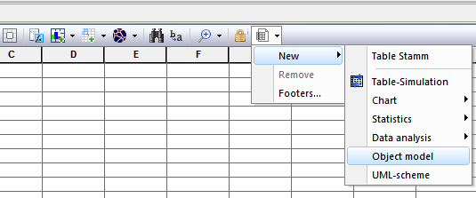
Figure 121. Creating the "Object Model" sheet from the ribbon

Figure 122. Creating the "Object Model" sheet from the toolbar sheets
The program can be supplied with ready-to-use components of object models or they can be created independently, as described below.
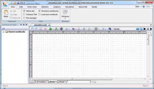
Figure 123. New sheet of the Object Model workbook
Editing the model
The elements of the object model are vector graphic elements that can be drawn by the user using the Stamm tools or loaded into the model from among the previously saved media. In addition, the functions of copying and pasting items via the Windows clipboard work. The model components are moved across the model canvas by dragging the mouse or using the cursor keys on the keyboard. The object model is saved on the media along with the workbook. The visual model is edited using the "Model" tab (Figure 123). Work with individual elements of the model are presented below.Working with model elements
Components of the system dynamics model
These elements are designed to organize the modeling of processes and systems. Each of the elements can be placed on the canvas of the object model using the drop-down menu of the "Components" button by selecting from the "System Dynamics" submenu Fig. 124.
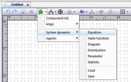
Figure 124. Inserting components of the system dynamics model
The Equation component
Externally, it can be any graphic element with several ports that are used to transmit equation parameters. (Fig. 125). The properties of the component can be changed if it is active by clicking on the "Components" drop-down menu button while using the dialog panel (Fig. 126).
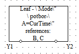
Figure 125. Component of the system dynamics model "Equation"
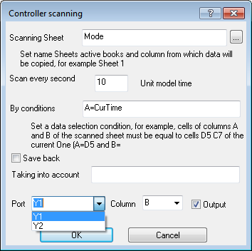
Figure 126. Properties of the Equation component
Сomponent "Table Function"
Externally, it can also be any graphic element with several ports that are used to transmit tabular values of the function. (Fig. 127). The function values are extracted from the Stamm worksheet table associated with the component. The properties of the component can be changed if it is active by clicking on the "Components" drop-down menu button while using the dialog panel (Fig. 128).
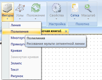
Figure 127. Component of the system dynamics model "Table Function"

Figure 128. Properties component "Table Function"
Diagram
It is a rectangle with a field sufficient to display graphical dependencies (Fig. 129). The properties of the component can be changed if it is active by clicking on the "Components" drop-down menu button while using the dialog panel (Fig. 130).
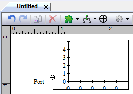
Figure 129. Component of the "Diagram" system dynamics model
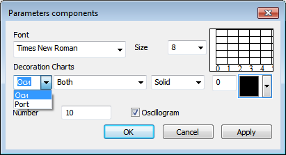
Figure 130. Свойства компонента «Diagram»
Distribution
It is an arbitrary graphic element with one port to which numerical data generated by the component is fed in accordance with a given distribution law of a random variable. (Fig. 131). Generated random numbers can be used by other components of the model via connection to the port. The properties of the component can be changed if it is active by clicking on the "Components" drop-down menu button while using the dialog panel (Fig. 132).
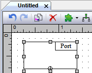
Figure 131. Component of the system dynamics model "Distribution"
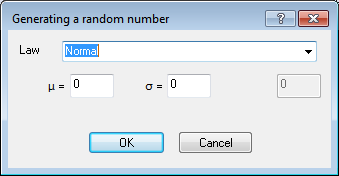
Figure 132. Properties of the "Distribution" component
Parameter
It is a rectangle with one port and a text numeric field with a field for changing the parameter. (Fig. 133). The parameter value is used by other components of the model through connection to the component port. The properties of the component can be changed if it is active by clicking on the "Components" drop-down menu button while using the dialog panel (Fig. 134).
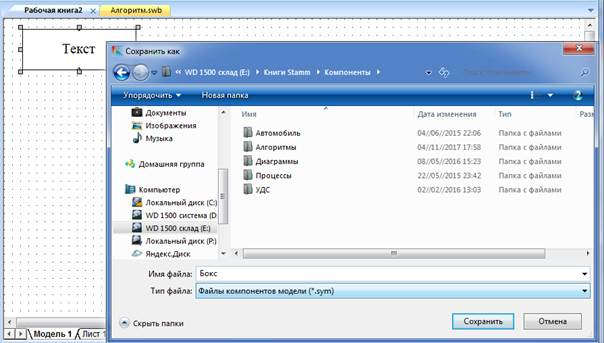
Figure 133. Component of the system dynamics model "Parameter"
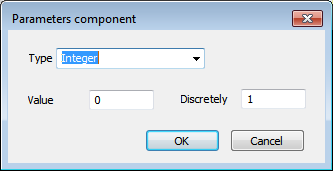
Figure 134. Properties of the "Parameter" component
Статистика
It is a rectangle with one port, half of which is occupied by a field for visualizing the distribution law of a random variable entering the input component (port), and the remaining part is a text field for displaying statistical parameters of a random variable. (Fig. 135). The properties of the component can be changed if it is active by clicking on the "Components" drop-down menu button while using the dialog panel (Fig. 136).
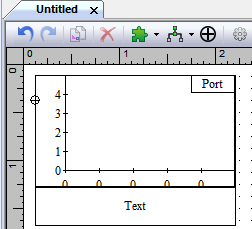
Figure 135. Component of the system dynamics model "Statistics"
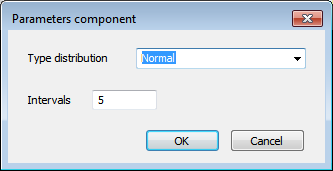
Figure 136. Properties of the "Statistics" component
Components of the agent model
These elements are designed to simulate the movement of independent agent entities in space. Each of the model elements can be placed on the canvas of the object model using the drop-down menu of the Components button by selecting from the Agents submenu Fig. 137.
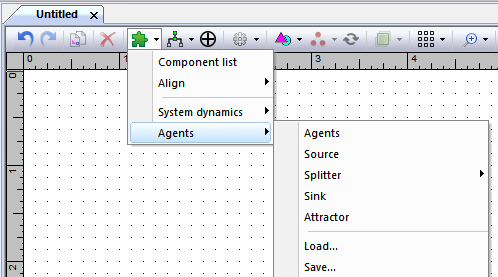
Figure 137. Inserting agent model components
The Agent component
A key element that any graphic element can be used to display. The properties of the component can be changed if it is active by clicking on the "Components" drop-down menu button while using the dialog panel (Fig. 139).
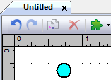
Figure 138. Component of the agent model "Agent"
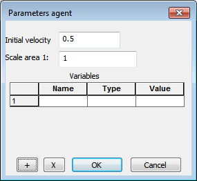
Figure 139. Properties of the Agent component
The "Agent Source"
The "Agent Source" is a component designed to generate agents and place them in the model, has one port for agents to exit. The properties of the component can be changed if it is active by clicking on the "Components" drop-down menu button while using the dialog panel (Fig. 141). At the same time, it is necessary to set a place on the canvas of the model where the agents injected into it (guides) will be placed. After entering the agent, it moves in accordance with the direction of the attractor.
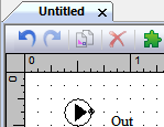
Figure 140. Component of the agent model "Source of agents"
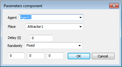
Figure 141. Properties of the Agent Source component
The component "Agent sink"
Component with the inverse function of the agent source is designed to remove agents from the model, has one port. The properties of the component can be changed if it is active by clicking on the "Components" drop-down menu button while using the dialog panel (Fig. 143). At the same time, it is necessary to set a place on the canvas of the model from where the agents (guides) will be removed. After removing the agent, it moves in accordance with the direction of the attractor.
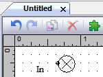
Figure 142. Component of the agent model "Agent Absorber"
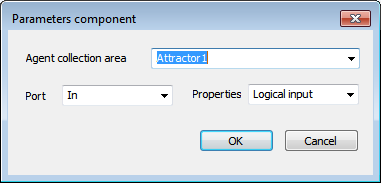
Figure 143. Properties of the Agent Absorber component
The "Splitter" component
The component is designed to control agent flows in the model, and can also perform the agent delay function. The number of ports of the component is determined by the user when entering it into the model using the context menu "Agents" - "Divider" (Fig. 144). The properties of the component can be changed if it is active by clicking on the button of the drop-down menu "Components" while using the dialog panel (Fig. 146). Using the properties panel, you can set a place on the canvas of the model from where the agents will come to the divider (guides), and also determine further directions of movement for each of the ports by attaching guides to them (Fig. 146).
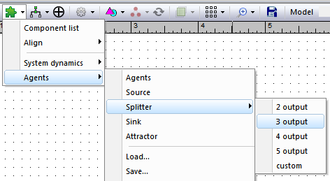
Figure 144. Entering the " Splitter " component into the model
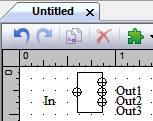
Figure 145. Component of the agent model " Splitter "
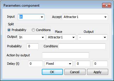
Figure 146. Properties of the " Splitter " component
The "Attractor" component
The component is designed to set the trajectory of agents in the model space and is a graphic element – a line, polyline, arc or their composition, bounded on both sides by ports (Fig. 147).

Figure 147. The component of the agent model is the "Attractor"
Relationship between components of the object model
Components of the "System Dynamics" type must be logically interconnected through ports for exchanging parameters during the simulation process. These connections are organized by connecting ports with a directional line, the type of which is selected from the context menu of the toolbar of the sheet of the object model "Connections" (Fig. 148). After selecting the desired type of connection, the mouse cursor is placed on the port of the first connected source element, after one left–click the line stretches to the destination port, the input is completed by clicking on the indicator port (fig. 149).
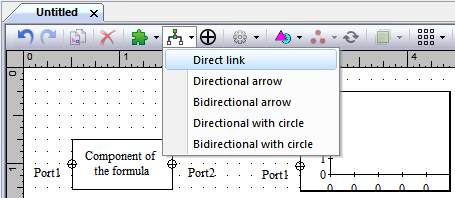
Figure 148. Choosing the relationship between the model components

Figure 149. Edit links
Graphic primitives
These elements are designed to visually display the components of the model being created and are vector images. They can be obtained by drawing on the canvas of the model using the mouse manipulator using techniques and methods that are standard for visual image editors. In addition, they can be placed on the canvas of the model by loading previously saved images from the selected media. First, you need to determine the desired type of the resulting element by selecting the appropriate tab from the drop-down menu of the "Shapes" button (Fig. 150).
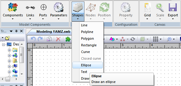
Figure 150. Selecting the shape type
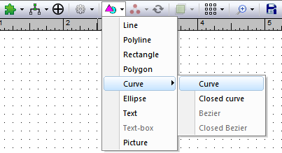
Figure 151. Selecting the shape type from toolbar sheets
One of the "Text" shapes is a rectangular box, inside of which is a test field (Figure 154).
Text notes can be placed outside and inside another shape and grouped with it, in this case we get at the disposal of the model component. For a better perception of the text field inside the component, you need to remove its framing using the properties panel.
To fully use the component when creating structural models, you also need to add and group ports and connections with it. Keeping in mind the different types of components, the number of graphic shapes and ports in the created component can be different and is determined by its required appearance and the number of required connections with other elements of the model.
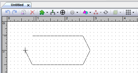
Figure 152. Drawing the "Polyline" graphic figure
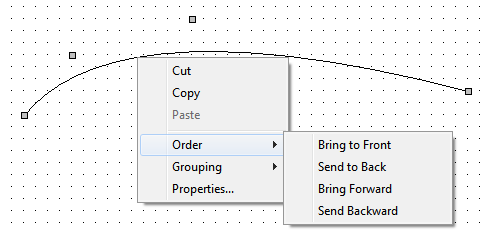
Figure 153. Context menu of the "Curve" graphic figure
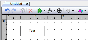
Figure 154. The "Text" graphic figure»
Ports
Ports are used to organize external links between the component being created and other elements of the model. Graphically, they are represented as a circle of small diameter (Fig. 127). The creation of ports available when you click the "Ports" tab "Components model". The port is placed in the desired location of the graphic shape, after which they must be grouped together for sharing as components of the model. Shapes that have ports can be connected using various types of connections (see below).
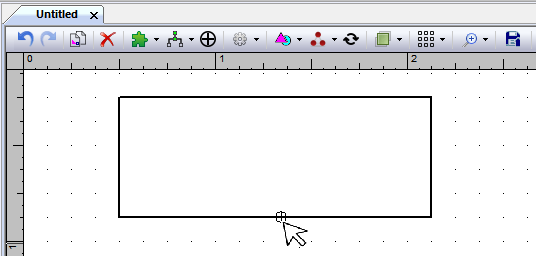
Figure 155. Creating a port for the "Rectangle" graphic shape
Uploading the component to the media
The created component can be saved on the media for the convenience of its further use when creating object models. To do this, you need to create one or more graphical primitives that will visually represent the component, and the required number of ports for communication. For the first of the created primitives, it is necessary to set a name according to the type of the component being created (Fig. 156). In the case of system dynamics components , these are.
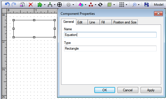
Figure 156. Changing the name of the primitive "Rectangle" to "Equation"
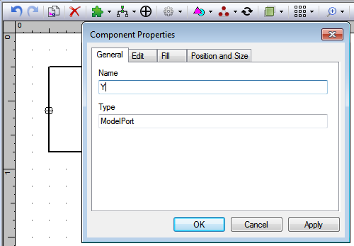
Figure 157. Changing the name of the port
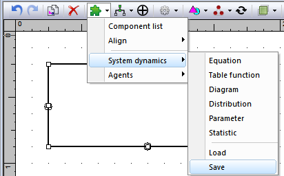
Figure 158. Unloading the component to the media
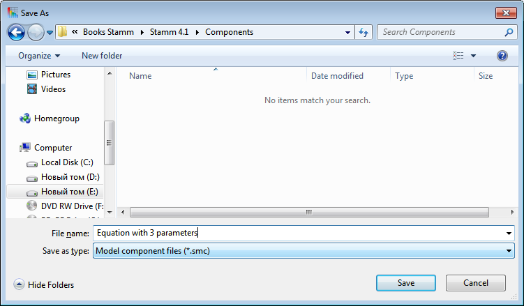
Figure 159. Saving the created component on the media
Loading a component into a model
Grouped elements that were previously saved on the media can be used when creating structural models, for which you need to use the "Components" button in the "Model Components" panel of the application ribbon. Then, in the dialog panel (Fig. 157), select the folder with the corresponding set of components, select the desired name and click "Open", then place the mouse cursor in the desired location of the model canvas and click with the left mouse button.
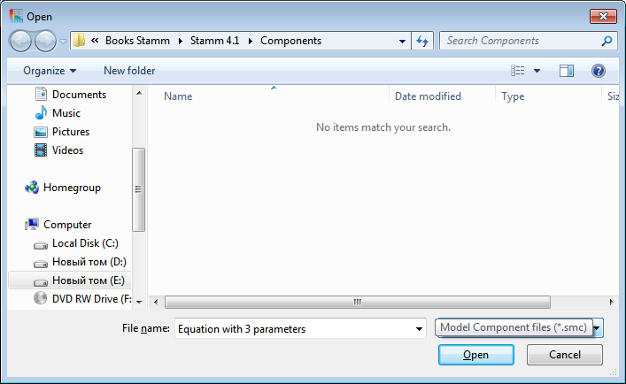
Figure 160. Loading a component from a data carrier
The use of model components
The creation of connections between the components
Components of the model are combined in the schema, or structure by creating a relationship between them. To do this, use the menu of the "Links" button on the "Model Components" tab. In the nested menu, select the desired type of connection, then the mouse cursor is placed on the desired port of the first of the components between which the connection is established. After a single click of the left mouse button, the communication line is extended to the corresponding port of the second component and the left button of the manipulator is pressed again (Fig. 158).
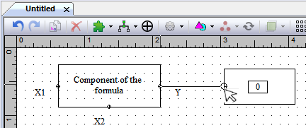
Figure 161. Creating a link between components
– terminates when connecting to the destination port;
– directional arrow-pointer at the point of connection to the second port;
– bidirectional arrow - contains pointers to both ports of the United;
– directional with a circle-draws a circle at the connection point to the second port;
– bi-directional with the circle draws a circle on both connected ports.
When model components with established relationships are moved together, the connection between them is maintained automatically.
Control points
There are nine control points on each component. They are arranged around the bounding box of the component: one at each corner, one in the middle of each side, and one in the center of the component. The control points establish the basis for spatial manipulations, such as rotation and scaling. The points along the edges of the bounding box are also used as default grab handles.Handles
Handles or nodes appear on the component when the user selects it. These elements allow the user to see what is selected, and then scale the component or move its vertices.On most pen components, these are the eight control points at the edges of the rectangle. However, for lines and curves, the markers are displayed on the vertices of the component, allowing the end user to move them.
You can set any graphical primitive to the "Edit vertices" mode, so that the markers are displayed only on individual vertices of the component, which allows the user to change their shape.
Editing the list of components
In order to view and edit components without moving around the model canvas, you need to use the "List of Components" menu of the "Components" button on the "Model Components"tab. The dialog box displays a list of the names and types of top-level components currently in the model. This allows the user to center the viewport by component or set of components, edit properties, and delete components (Figure 159).Resizing components
To align the geometric dimensions of several components without editing each of them individually, you can select them on the canvas and use the Align Size menu of the Components button on the Model Components tab. Or similar items in the same menu "Height" and "Width".Rotating components
To rotate the components, select them on the canvas and use the "Rotate Right" menu of the "Position" buttons of the "Shapes" tab. Or similar items in the same menu "Turn left", "Flip horizontally" and "Flip vertically". To rotate the component at any angle, click on the "Position" button in the "Shapes" tab and, moving the mouse cursor to the desired shape, click the left button and, without releasing it, rotate the component to the desired angle and release the mouse button.
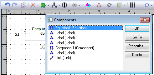
Figure 162. List of object model components
The relative position of the components
The visibility of the components is determined by their relative position in Z-dimensional space. In order to correctly position the desired component, you can use the context menu of the component, called by right-clicking, where you can select the "Order" option . The following options are available here: "To the foreground", "Move forward", "Move Back", and "To the background".Combining components
Individual components and graphical primitives, as well as ports, can be combined into a single block. To do this, select the objects to be combined on the canvas, and then use the right-click context menu, where you can select the "Grouping" option. Here the options are available: "Group "and" Ungroup.Working with the object model canvas
Configuring the canvas
Background color
The canvas background color is supported by the model. By default, the model's background color is white. In the viewport, the background color is used to fill the canvas before rendering the components. If a single color scheme is not enough for the background, you can assign a background component to the model. The background component appears behind all other canvas components and cannot be directly edited by the user.Canvas parameters
For a canvas, you can configure settings that make it easier to create structural models on it, such as turning the grid on or off. Setting the canvas parameters is performed by calling the context menu when right-clicking outside the components (Fig. 160.
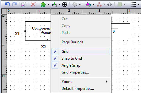
Figure 163. Managing the model canvas
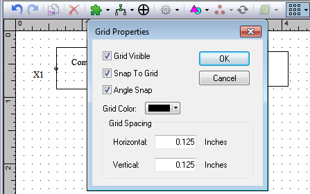
Figure 164. Configuring grid properties
Export files
This feature allows the user to export the canvas to a file using one of several common image file formats. The program currently supports exporting files for Windows in the extended metafile format and several bitmap image formats. The Extended Metafile format is a vector graphics format supported by most Windows drawing programs.The system also supports export to bitmap image formats of the following types.
Hardware-independent Windows bitmap (DIB or BMP).
JPG (JPEG file sharing format).
PCX (PC Paintbrush).
GIF (graphic interchange format).
TGA (Targa image file).
TIFF (image file format with tags).
To export to a file, click the Export button on the Model tab of the ribbon and select the appropriate file type.
Modeling management
The preparation of the components of the object model, the installation of the necessary logical connections is carried out in the worksheet of the workbook "Object Model" (Fig. 123). Modeling parameters are set using the "Parameters" button on the toolbar of this sheet, while using the dialog panel (Fig. 165).
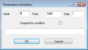
Figure 167. Setting modeling parameters
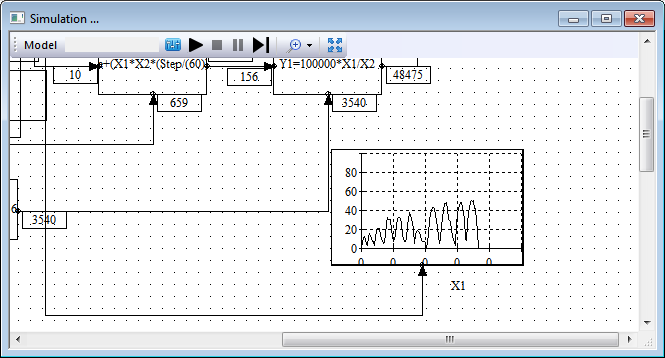
Figure 168. Simulation Experiment Window
