Stamm

EXAMPLES OF WORKING WITH DATA
Each of the examples is accompanied by a description and a link to the workbook with the implementation.

Using simulation models of tabular type

Modeling of expenses related to car sales in the salon Upload

The following example from the practice of a car dealership is posted on the Internet. In the last hundred months, the sales volume at the dealership ranges from 5 to 11 new cars per month. The salon manager orders 25 cars each time and makes a new order when the stock in the store is reduced to 10 cars. A new order can be made only after the previous one has been completed. We will simulate this strategy for 24 months. Let's perform a Monte Carlo simulation by setting car sales for a month by a random number with the given parameters of the distribution law.
We believe that:
a) the initial stock is 30 cars
b) the cost of storing one car is 550,000 rubles per month.
c) one missed sale brings an average loss of 3,330,000 rubles.
d) one order costs 500,000 rubles.
Modeling tasks:
1. How many orders will have to be made in two years?
2. What are the costs associated with this strategy (thousand rubles)?
Let's create a new workbook and insert a simulation sheet there. Let's call it "Imitation of sales". In this sheet, we will create 6 special controller cells necessary for sales modeling (Fig. 9.12).
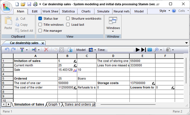
 
Figure 9.12. Simulation sheet for sales modelling
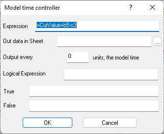
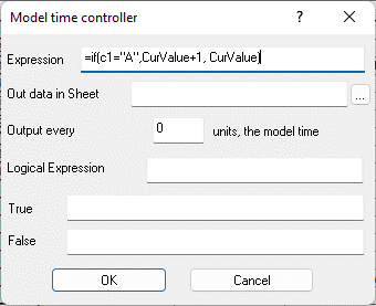
The first cell B1 – controller "Calculated expression" is designed to simulate the number of cars of this brand in the cabin. The properties of the cell are shown in Figure 9.13.

 
Figure 2. Formula in cell B1

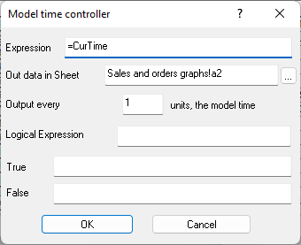
All special cells are recalculated at each iteration, that is, the change of the calendar month. At the same time, the number of ordered cars is added to the current value in cell B1, if there is an order, and the number of cars sold, generated randomly, is subtracted. Cell B2 – controller "Calculated expression" is designed to set the value of the current month. The properties of the cell are shown in Fig. 9.14.

 
Figure 9.14. Formula in cell B2

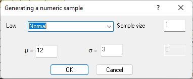
Cell B3 – controller "Random variable Generator" is designed to simulate the sales of the current month. The properties of the cell are shown in Fig. 9.15. The cell will be a generator of a random value of sales in the current month, which is subject to the normal law with the parameters expectation - 12 and variance 3.

 
Figure 9.15. Formula in cell B3

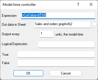
Cell B7 – controller "Calculated expression" is designed to simulate the costs of ordering cars. The properties of the cell are shown in Fig. 9.16.

 
Figure 9.16. Formula in cell B7

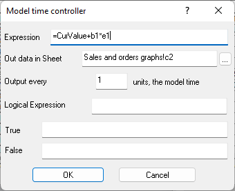
Cell E6 is designed to simulate the cost of storing cars in the cabin. The properties of the cell are shown in Fig. 9.17.

 
Figure 9.17. Formula in cell E6

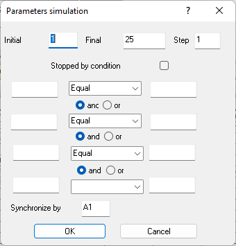
The last special cell F7 is designed to simulate losses from the refusal to sell a car. The properties of the cell are shown in Fig. 9.18. The model parameters are set via the dialog panel (Fig. 9.19). At the same time, the current month is used as a model time variable, respectively, the modeling step is 1. In order to simulate the operation of the salon for two years, the final value is set to 25, when it is reached, the simulation stops.

 
Figure 9.18. Formula in cell F7

 
Figure 9.19. Model Parameters
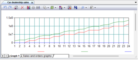
In the properties of the cells that store the values of the current month and accumulated costs, the output of numerical values is set at each step of the modeling in the workbook "Sales and Order Schedules" (Fig. 9.16 – 9.18). Accordingly, after the end of the model, you can select a data block in this sheet to get a graph of cost changes by elements on a separate graphical representation (Fig. 9.20). The operation of the model stops when the specified model period is reached (Fig. 9.21).

 
Figure 9.20. Cost change graphs

 
Figure 9.21. Simulation results

Modeling of repair of mechanisms in the workshop Upload

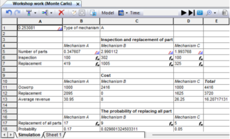
The repair shop performs preventive inspection and repair of some mechanisms. Of all the mechanisms received by the repair service, 30% are mechanisms of type A, 50% – type B, 20% – type C. The mechanism of type A includes 10 parts that require inspection; the mechanism of type B includes six such parts, type C – four parts. The number of parts requiring replacement in each of the mechanisms can be any. For example, in a type A mechanism, the number of parts requiring replacement can range from 0 to 10 (with the same probability). For each replaced part, the customer pays the repair shop 5 den. units. In addition, the customer pays 10 monetary units for the inspection of mechanism A. units, for the inspection of the mechanism B – 8 monetary units, for the inspection of the mechanism C – 14 monetary units. Create an algorithm and a program (based on the Monte Carlo method) to determine the following values: – the probability that all parts will need to be replaced in the mechanism; – the average revenue of the workshop from the inspection and repair of one mechanism. The problem was solved using a macro written in VBA for Excel, implementing the Monte Carlo method. The implementation of this task in the Stamm system is presented below. The simulation sheet of the corresponding workbook contains 4 controller cells, which are random number generators distributed according to a given law, and 9 controller cells "Calculated expression" (Fig. 9.22).
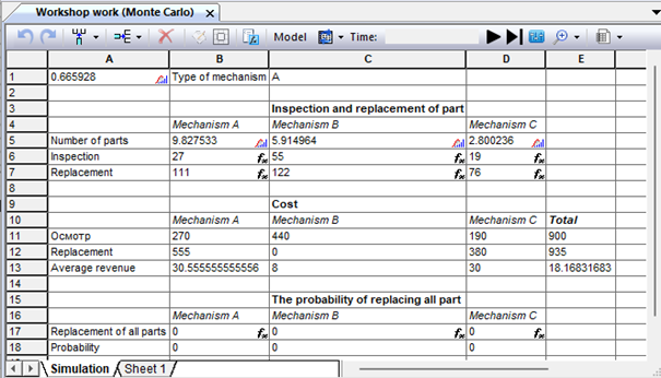
 
Figure 9.22. The sheet of simulation of inspections and replacement of parts
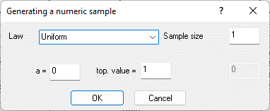
Cell B1 generates a uniformly distributed random variable in the range from 0 to 1.

 
Figure 9.23. Controller cell B1

After that, the formula in cell C1 selects the mechanism code depending on the value of the variable generated in B1 =IF(A1<0.3,"A",IF(A1<0.8,"B","C")) Depending on the code received as a result of the iteration, one of the controller cells increases the counter of the mechanisms received for inspection by one. Figure 9.24 shows cell B6, which is responsible for counting the number of examined type A mechanisms.

 
Figure 9.24. Formula in cell B6

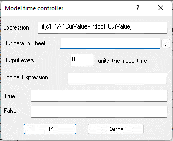
Cells C6 and D6 contain similar formulas and are responsible, respectively, for counting the number of examined mechanisms of type B and C. Replacement of parts for each type of mechanism is imitated by cells B7, C7, D7 using the same type of formulas (Fig. 9.25), increasing the value in the cells for their type. And the number of replaced parts by types of mechanisms is generated in cells B5, C5, D5 according to the same uniform distribution law (see Fig. 9.26).

 
Figure 9.25. Formula expression in cell B7
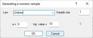
 
Figure 9.26. Generation of a random variable in cell B5
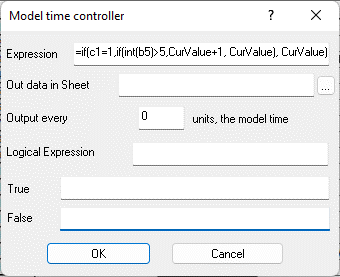
Cells B17, C17 and D17 track the number of replaced parts generated in cells B5, C5, D5, compare it with the maximum number of parts in the mechanism of the corresponding type and increase the counters of complete replacement by types of mechanisms (Fig. 9.27).

 
Figure 9.27. Formula in cell B17

 
Fig. 9.28. Simulation results

Formulas in ordinary cells of the sheet use the values generated during the simulation to calculate the necessary indicators. Calculation of the cost of inspection of mechanisms by types A, B, C is carried out in cells B11, C11 and D11 according to the formulas, respectively: =10 *B6, =8*C6, =10*D6. The cost of replacing parts by types of mechanisms is calculated in cells B12, C12 and D12 according to the formulas: =5*B7, =5*B7, =5*D7. The average revenue from the mechanisms for the simulated period is calculated in cells: =(B11+B12)/B6, =(C11+C12)/C6, =(D11+D12)/D6. And finally, the probability of a complete replacement is calculated based on the number of complete replacements of parts by type of mechanisms and the total number of inspections of mechanisms of each type according to the formulas: =B17/B6, =C17/C6, =D17/D6.